There are different ways of doing animations - the simplest is to have each mesh associated with a transform (matrix) - you update the transform and the mesh moves around (scaled, rotated and translated). However, this makes it difficult to create soft body effets - with smooth surfaces.
Skinned animations is a mixed of rigid skeletons and a mesh surface - similar to the human body - we have a skeleton under our body - as the skeleton moves so the skin on the surface. The animation principle for skinning is very similar - we create a rigid skeleton (called nodes) - each of which have a transform - we animate these using animation frames.
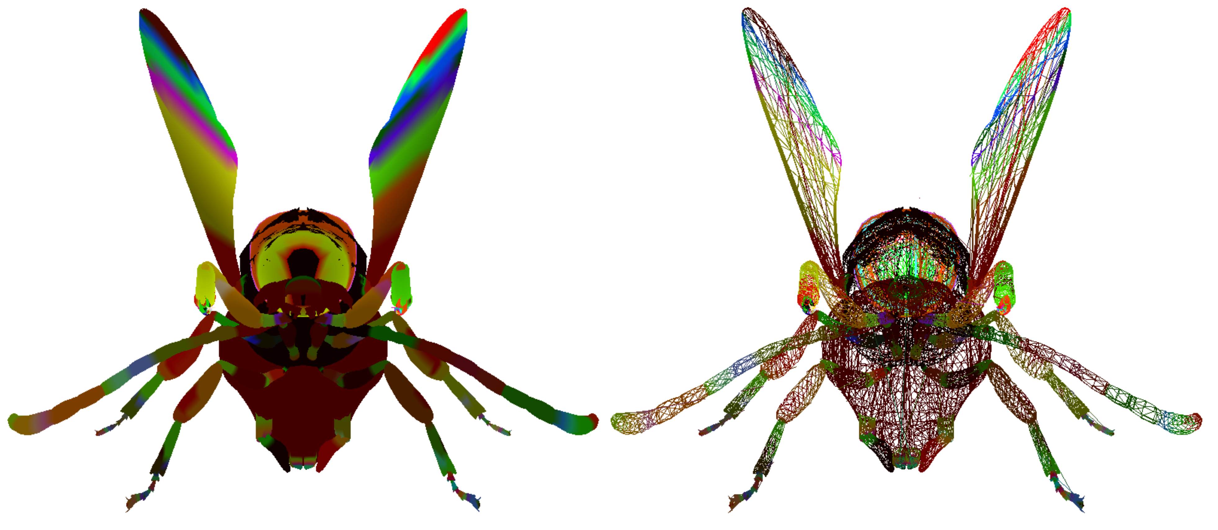
The Bee in the image below shows a single mesh which is getting animated by 112 bones - the different colors indicated the areas of the mesh which are influenced by different bones.
Skinned Bee model, the colors help show the bone/weight influence areas for the mesh.
The `skin` is a mesh which `links` to the skeleton. However, instead of a single transform for each mesh, we have a transform for each vertex! Not just one transform, but typically 4. We average between the multiple transforms to create `smooth` deformations (when two vertices next to each other are influenced by different transforms they don't just snap or change sharply).
The model data for this tutorial uses a simple insect with wings - both the binary and ascii versions:
• Models (.glb) (Bee.glb ) • Models (.gltf) (Bee.gltf)
Details about the model:
Number of Meshes: 1
Number of Nodes: 112
Number of Materials: 1
Number of Textures: 5
Number of Animations: 3
Number of Skins: 1
At this point, we need to load:
1. mesh (collection of vertex data - includes positions, joint indexes and weights)
2. joint data (hierarchy/skeleton/nodes)
3. animatoin data (control/move the joints)
The concept of skinning might seem like a lot of work - adding extra transform data to each vertex - when you've got a complex skinned model with hundreds of thousands of vertices - it might seem impossible? However, with tools like Blender or Maya; it's easy to setup the skinned mesh/file data - these specialist modeling packages help manage the complexity of designing and setting the weights so the final animated data is perfect.
Loading in the Mesh Data
The mesh for the Bee is a single set of vertex data (single mesh) - you can have multiple meshes/animations/skins inside a glTF file - but for this example, we have only a single mesh/skin.
<?php
Mesh 0 - Name: Mesh_0
   Primitive 0:
      PrimitiveMode: 4   // 4 is the default for triangle list in glTF meshes
      Number of Vertices: 29635
      Number of Indices: 155193
      ...
If we look at a few of the vertices for the positions and indices, these are what we'd expect for any mesh:
Dump the first 12 vertex values
<?php
Vertex Position 0: 1.47, 5.96, 5.64,
Vertex Position 1: 1.41, 6.01, 5.51,
Vertex Position 2: 1.30, 6.08, 5.64,
Vertex Position 3: 1.36, 6.04, 5.80,
Vertex Position 4: 1.23, 6.08, 5.47,
Vertex Position 5: 1.35, 6.04, 5.44,
Vertex Position 6: 1.35, 5.34, 4.70,
Vertex Position 7: 1.47, 5.51, 4.90,
Vertex Position 8: 1.49, 5.36, 4.80,
Vertex Position 9: 1.30, 5.52, 4.79,
Vertex Position 10: 1.63, 5.45, 5.01,
Vertex Position 11: 1.63, 5.30, 4.90,
Vertex Position 12: 1.75, 5.19, 5.00,
....
Now, let's dump the first 12 indices values (triangle index list):
<?php
Indices Triangle 0:  0, 1, 2,
Indices Triangle 1:  2, 3, 0,
Indices Triangle 2:  4, 2, 1,
Indices Triangle 3:  4, 1, 5,
Indices Triangle 4:  6, 7, 8,
Indices Triangle 5:  7, 6, 9,
Indices Triangle 6:  8, 10, 11,
Indices Triangle 7:  10, 8, 7,
Indices Triangle 8:  12, 11, 13,
Indices Triangle 9:  11, 10, 13,
Indices Triangle 10:  14, 15, 16,
Indices Triangle 11:  15, 14, 17,
Indices Triangle 12:  18, 19, 20,
...
These seems logical and correct (we're limiting the vertex data with floating point alues to 2 decimal places).
Now for the joint indices and weights - which are stored with the mesh data.
The joint indexes are stored as unsigned integers (not floating points) - and the index values should be within the joint range (i.e., 0 to number of joints - 1).
As there are thousands of vertices, let's dump the first 12, plus a few other ones later on - so you can see the values change.
<?php
Vertex Joint Index 0: 2, 0, 0, 0,
Vertex Joint Index 1: 2, 0, 0, 0,
Vertex Joint Index 2: 2, 0, 0, 0,
Vertex Joint Index 3: 2, 0, 0, 0,
Vertex Joint Index 4: 2, 0, 0, 0,
Vertex Joint Index 5: 2, 0, 0, 0,
Vertex Joint Index 6: 2, 0, 0, 0,
Vertex Joint Index 7: 2, 0, 0, 0,
Vertex Joint Index 8: 2, 0, 0, 0,
Vertex Joint Index 9: 2, 0, 0, 0,
Vertex Joint Index 10: 2, 0, 0, 0,
Vertex Joint Index 11: 2, 0, 0, 0,
Vertex Joint Index 12: 2, 0, 0, 0,
...
Vertex Joint Index 2816: 88, 89, 0, 0,
...
Vertex Joint Index 3072: 93, 92, 94, 0,
...
Vertex Joint Index 3584: 90, 91, 0, 0,
...
Vertex Joint Index 3840: 93, 94, 95, 92,
....
We have the same number of weights as we do joints. A very important point to note - is the weights for each vertex should add up to 1.0.
These values can be loaded into GPU buffers and passed to the vertex shader - for testing we can just render the mesh as we would any other mesh without the influence of the joints/weights. If the vertex data is correct the mesh should be shown on screen.
Vertex code snippet showing the vertex data being used without any skinning:
that means the transforms has zero impact on the output and is nulled out.
Bone (or Joint) Data
Let's move onto the bones. We load the bone data in; and is nothing more than an array of transforms. These can be matrices or a mix - however, for animated bones local transforms as a position, scale and rotation - these are easier to interpolate between than matrices.
The glTF file format refers to the bones (or joints) as `nodes`.
For the Bee model, there are 112 nodes - that means their is 112 joints! (however, that does not mean all of them will be used for the skinned animation, but we need to load them all).
Loading and dumping the node data we would see this:
Dumped the first 5, plus node 107 - to show the variety of information. Important to note the nodes provide hierarchical information - which children are connected to each node. The transform for each node is a local transform only - so to get the world transform (which is what we need) we have to combined all the transforms from each child.
If we load all the nodes and connect them together in a hierarchy, we get something like this (use indentation to represent a 'child'):
For the Bee model - everything is connected to the root node - however, this isn't a rule - you can have multiple root nodes - each with their own hierarchy! Just somethinig to be aware of if you try more complex animations/files/examples.
We construct a local matrix for each node (using the transform from each node). This is the `default` hierarchy transform for the idle test post (without any animation).
As the local transform is now a matrix for each node, we can recurse the hierarchy and build the world transform for each node. We start at the root and pass the transform down the hierarchy.
We do this in two parts:
1. Build the hierarchy
2. Update the hierarch with 'world' transforms
First, let's build the hierarchy from the array of nodes:
<?php
    // 'nodes' variable is an array of all the nodes loaded in earlier, build the hierarchy
    // use the node indexes

    function buildHierarchy(nodeIndex, nodes) {
        // Get the current node
        let node = nodes[nodeIndex];

        if (!node) {
            console.error(`Node at index ${nodeIndex} not found!`);
            return null;
        }

        // Recursively build children hierarchies
        let children = (node.children || []).map(childIndex => buildHierarchy(childIndex, nodes));

          let localmat = mat4.create();
        {
              if ( node.matrix )
            {
                mat4.copy(localmat, node.matrix);
            }
              else
            {
                  let scale       = node.scale ? node.scale : [1,1,1];
                let rotation    = node.rotation ? node.rotation : [0,0,0,1];
                let translation = node.translation ? node.translation : [0,0,0];

                  let rotMat   = mat4.create();
                let scaleMat = mat4.create();
                let transMat = mat4.create();
                rotMat   = mat4.fromQuat(mat4.create(), rotation);
                scaleMat = mat4.fromScaling(mat4.create(), scale);
                mat4.translate(transMat, mat4.create(), translation);

                  mat4.multiply(localmat, localmat, transMat);  // Finally translation
                mat4.multiply(localmat, localmat, rotMat);    // Then rotation
                mat4.multiply(localmat, localmat, scaleMat);  // Scale first


            }

        }

        // Return the node with its hierarchy
        return {
            index: nodeIndex,
            name: node.name || `Unnamed Node ${nodeIndex}`,
            localmat: localmat,
            worldmat: mat4.create(),
            // other information for each node (e.g., animation transforms)
            children: children,
        };
    }
Second, let's construct the world transform for each node using the parent-child relationship fo the hierarchy:
<?php
    function updateHierarchyMatrices(node, parentMatrix) {

        // Add in the animation transform data here later on

        // combine the local matrix with the parent
          mat4.multiply(node.worldmat, parentMatrix, node.localmat  );


        // Recursively print children (pass this world matrix to the child)
        (node.children || []).forEach(child => updateHierarchyMatrices(child, node.worldmat));
    }
This gives us a hierarchy with transforms both in local and world space.
At this point, we've done a lot of work - but this is the step that hits most people hard - the inverse transforms! The transform for each node is in node space - and our vertex position is in mesh space.
We don't need to animate the inverse transforms to convert the vertex position to the joint space - so an array of inverse transforms is stored on the mesh.
Inverse Transforms
Each skin has an array of inverse transforms as an array of matrices (mat4x4) which we can load easily.
For example, loading the inverse matrices from the glTF file:
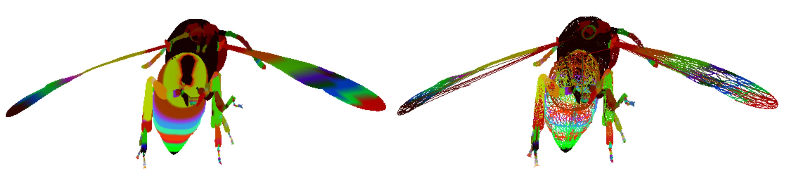
Default pose view using the node transforms (no animation data). Combines the inverse matrix with the node transform and is passed to the vertex shader which uses the weights/node indexes. View shows the solid and wireframe view - debug view so the depth buffer isn't enabled.
Animation Data
The animation data is the transform for each node that will replace the default node data. Important we don't combine it with the transform on the node, but replace it.
The animations are stored on their own in the glTF file - so we can loop over the animation data and get the timing information (e.g., maximum duration of the animation).
<?php
let maxDuration = 0;

parsedData.animations.forEach(animation => {
  animation.details.forEach(detail => {
    const sampler = animation.samplers[detail.samplerIndex];

    // Get the duration for this specific sampler
    const samplerDuration = sampler.inputData[sampler.inputData.length - 1];

    // Check if this duration is the maximum
    if (samplerDuration > maxDuration) {
      maxDuration = samplerDuration;
    }
  });
});

return maxDuration;
We can have any number of animations and within each animation is a set of
samples
. The sample is like a keyframe - so at that keyframe it can provide one or more position, rotation and scale transforms.
The samples are NOT equally spaced out - and use a time value - so we need to keep track of the prevous time and transform and interpolate between them.
The following provides an example of looping over the animations and calculating the transform for the node for a given time. If we have a currentTime of 2.0 - calculate the transform for that node.
We calculate the previous and current sample indexes and interpolate between them using the currentTime value.
We sample keyframe is linked to a node (using an index) - we store the animation transform on each node as
animTMat
,
animSMat
and
animRMat
for translation, scaling and rotation.
Remember, it might only have a translation transform or a rotation - it does not need to have all three;
<?php
parsedData.animations.forEach( (animation, animIndex) => {
    animation.details.forEach(detail => {

          let hnode = findHierarchyNode( hierarchy, detail.index );
          if ( !hnode )
        {
            console.warn('**unable to find animation node!!**', detail);
            return;
        }

        const sampler = animation.samplers[detail.samplerIndex];

        // Get the duration for this specific sampler
        const samplerDuration = sampler.inputData[sampler.inputData.length - 1];
        let samplerTime = currentTime;

        // Each sampler can have a different end time
        samplerTime = clamp(samplerTime, 0.0, samplerDuration - 0.001);

        // Find the current frame and next frame
        let currentFrame = 0;
        for (let i = 0; i < sampler.inputData.length - 1; i++) {
            if (samplerTime < sampler.inputData[i + 1]) {
                currentFrame = i;
                break;
            }
        }
        const nextFrame = (currentFrame + 1) % sampler.inputData.length;

        // Get time values for current and next frames
        const currentTimeValue = sampler.inputData[currentFrame];
        const nextTimeValue = sampler.inputData[nextFrame];
        const deltaTime = Math.max(nextTimeValue - currentTimeValue, 1e-6);


        let interpolationFactor = (samplerTime - currentTimeValue) / deltaTime;
        interpolationFactor = clamp(interpolationFactor, 0, 1);

        const outputLength = detail.path === 'rotation' ? 4 : 3;
        const startOutput = sampler.outputData.slice(currentFrame * outputLength, (currentFrame + 1) * outputLength);
        const endOutput = sampler.outputData.slice(nextFrame * outputLength, (nextFrame + 1) * outputLength);

        const interpolatedOutput = startOutput.map((start, i) => {
            const end = endOutput[i];
            if (isNaN(end) || isNaN(start)) {
                console.warn('Encountered NaN in animation output data.');
                return start; // Fallback to start if NaN encountered
            }
            return start + (end - start) * interpolationFactor;
        });

        if (detail.path === 'translation') {
            let offset = interpolatedOutput.slice(0, 3);
            let translationMatrix = mat4.create();
            mat4.translate(translationMatrix, translationMatrix, offset);
              hnode.animTMat = translationMatrix;

        } else if (detail.path === 'rotation') {

            // Interpolate between the rotations and normalize (not SLERP)
            let len = 1.0 / Math.sqrt(
                interpolatedOutput[0] * interpolatedOutput[0] +
                interpolatedOutput[1] * interpolatedOutput[1] +
                interpolatedOutput[2] * interpolatedOutput[2] +
                interpolatedOutput[3] * interpolatedOutput[3]
            );
              if (isNaN(len) || len === 0) {
                console.warn('Invalid quaternion length.');
                return;
            }
            interpolatedOutput[0] *= len;
            interpolatedOutput[1] *= len;
            interpolatedOutput[2] *= len;
            interpolatedOutput[3] *= len;

            let rotationMatrix = mat4.fromQuat(mat4.create(), interpolatedOutput);
              hnode.animRMat = rotationMatrix;
        }
        // Handle scaling
        else if (detail.path === 'scale') {
            let scale = interpolatedOutput.slice(0, 3); // Expecting scale values for x, y, and z
            let scaleMatrix = mat4.create();
            mat4.fromScaling(scaleMatrix, scale);
              hnode.animSMat = scaleMatrix;
        }
        else {
            console.log('error unknown animation:', detail.path );
        }
    });
});
Now we have the animation transform on each node - we can modify the update hiearchy - instead of using the transform from each node - we use the transform from the animaton.
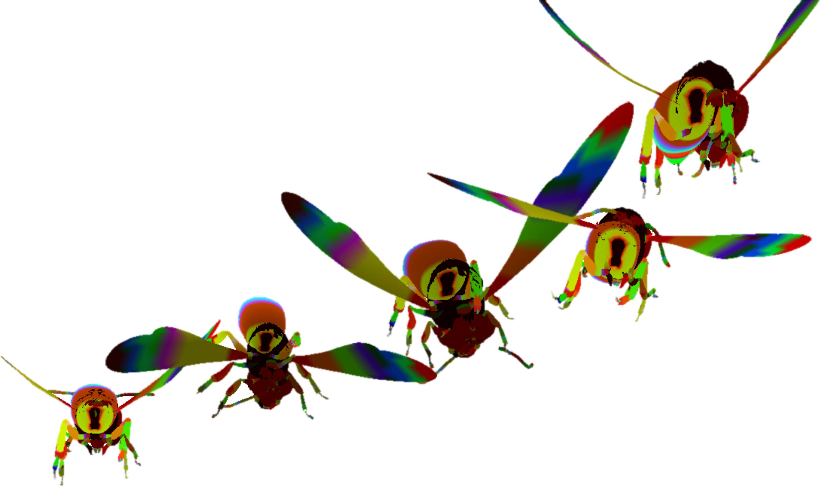
Draw multiple animation frames on top of one another showing the Bee moving around due to the animation. Flaps its wings and takes off - hovering and then coming down to land.
function updateHierarchyMatrices(node, parentMatrix) {
      let animmat = mat4.create();

    mat4.copy( animmat, node.localmat );

    // If we don't have animation data for this node - use the default - we need
    // to check if we this! Not all nodes are animated
    if ( node.animSMat  || node.animTMat || node.animRMat )
    {
       let animSMat = node.animSMat ? node.animSMat : mat4.create();
       let animTMat = node.animTMat ? node.animTMat : mat4.create();
       let animRMat = node.animRMat ? node.animRMat : mat4.create();


       animmat = mat4.create();
       mat4.multiply(animmat, animmat, animTMat);  // Finally translation
       mat4.multiply(animmat, animmat, animRMat);  // Then rotation
       mat4.multiply(animmat, animmat, animSMat);  // Scale first
    }

      // combine both local node matrix and animation matrix
    // VERY IMPORTANT - The animation transform data **replaces** the
    // transform data on the nodes (i.e., local transforms)
    // new set of transforms
      let tmp = mat4.create();

    mat4.copy( tmp, animmat );

    // combine the new local matrix with the parent
      mat4.multiply(node.worldmat, parentMatrix, tmp  );

    // Recursively print children - pass the local world to the children of this node
    (node.children || []).forEach(child => updateHierarchyMatrices(child, node.worldmat));
}
Use the currentTime of 5.0 - which moves the Bee position.
Things to Try
• The hierarchy animation has the Bee move around the screen - however, instead of having it fly around arbitarily - control it! Overide the base node position so you move the Bee around the screen programatically! Control it using the mouse cursor or cursor keys. Make it do loops or follow things around.
• Load in a 3d flower - and have the fly hover around the flower (override the position of the base node to control this)