You can simulation fluids in lots of different ways - using particles or springs! But if you want to do it so it's all swirly and juicy - and looks out of this world - then grid-based models are the way to go (along the lines of computational fluid dyanmics).
The reason it is often avoided - and makes people run for the hills is the Navier Stoke equations. They arne't pretty!
We're going to go through implementing it on WebGPU! We want it fast, realistic, interactive and runs in real-time!
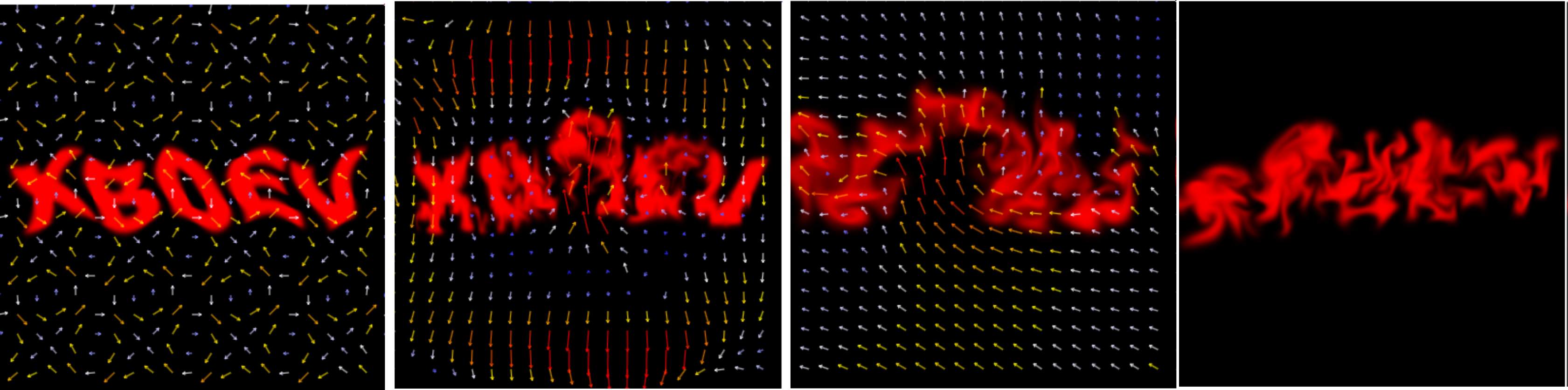
Fluid simulation output - see the die/color mixing - in addition to showing the velocity field.
Fluid Simulations - What? Go through what it all means...
Lets talk about whats happening and why...
We have a grid of values - and within each grid cell is some information.
Two pieces of information in each cell:
1. velocity and
2. die color.
As you'll notice from the figure below - the key pieces of information are the die (color) and the velocity which is reponsible for moving the die/color around. You could do a simple simultion with just these two values - but you'll notice it doesn't look realistic (just looks like it fades and scrolls - it lacks that swirling and mixing that you'd see when you look at a liquid in a glass).
Example of the program running - showing the interactive nature - start with a die in the pattern of some text.
Velocity Field
For any given point in the grid, we can access the velocity at that point using the x, y coordinate, this velocity value tells us the velocity of the fluid at that point.
Easiest way to think of the belocity field is the direction that things are moving, so if you have:
For instance, if every cell has a velocity
u(x,y)=(1,0)
- then it will appear to scroll to the right.
Advection - is when we use this velocity to move things about! If you’ve got some black dye in some water, and the water is moving to the right, then surprise surprise, the black dye moves right.
Of course, you can have very complex swirly velocities representing more complex currents - so the dye swirls and mixes in a more complex manner.
So you can imagine, if lots of cells each having a vectors; each pointing in different direction with different magnitudes - we'd have to try and keep track of what is going where! This can be complex and messy!
A better way is to take a cell - and look at the velocity vector for that cell - and look at where it came from - not where it is going.
So, instead of figuring out where our imaginary particles at the grid points go to, we'll figure out where they came from in order to calculate the next time step.
With this scheme, we only need to write to a single grid point, and we don't need to consider the contributions of imaginary particles coming from multiple different places.
The last teensy hurdle is the value from where it came from might not be at an exact grid point. For instance, it comes from (x=10.2,y=33.5). We use a bilinear interpolation on the surrounding 4 grid points instead of just picking the value rounded to the nearest digit. If we just use the rounded value - the liquid becomes unstable and noisy and doesn't move smoothly as we want.
Advecting the die is easy and straightforward - and we can test the advect function is working - by watching the die color scroll in the direction of the velocity.
In addition to advecting the die color, we also advect the vector itself! Just as the ink would move through the fluid, so too will the velocity field itself!
Divergent Fields (Keep Density)
This is where it gets complex :( Water is roughly incompressible. That means that at every spot, you have to have the same amount of fluid entering that spot as leaving it.
If we just use the advection - and the vectors push against each other - the die would disapear - it would be squashed into nothing! It emulates the pressure/density characterists of liquid - this is what gives us those swirly characteristics.
Mathematically, we can represent this fact by saying a field is divergence-free. The divergence of a velocity field (u) is a measure of how much net stuff is entering or leaving a given spot in the field.
An incompressible fluid will have a divergence of zero everywhere. So, if we want our simulated fluid to look kind of like a real fluid, we better make sure it's divergence-free.
This is the point that brings in the Navier-Stokes equations which describe the motion of fluids! These equations can be scary - especially if you're not comfortable is differential equations and solving for unknowns ;)
Calculating Divergence
The divergence of a velocity field \( \vec{u} \), denoted as \( \text{div}(\vec{u}) \) or \( \nabla \cdot \vec{u} \), measures the net rate at which "stuff" is entering or leaving a specific location in the field. For a 2D velocity field, it is defined as:
At this point, it’s helpful to remember that, for the purposes of the simulation, we're not interested in knowing the value of pressure - we just need to calculate it to solve our problem.
We're dealing with a discrete system - with approximate steps for the cells - so it won't be exact - but it'll be close enough to help stear our solution the the right direction.
We want to know about its approximate value to correct the velocities at the grid points.
The goal is to calculate the pressure \( p \) on a grid, where \( \epsilon \) is the distance between adjacent cells. For each grid point \( (x, y) \), we form one equation with 5 unknown pressure values, based on the velocities at surrounding points. If the grid has \( n \times m \) locations, this leads to \( n \times m \) equations.
Using cleaner notation, we define \( p_{i,j} \) as the pressure at grid point \( (i, j) \), and group known values into a divergence term \( d_{i,j} \). The system of equations is simplified as:
We can't get the best solution in a single calculation - too many unknowns - instead, we can use a iterative approach to find a best guess solution.
The iterative method of solving this system of equations, where each iteration provides values closer and closer to a real solution (use the Jacobi Method).
In the Jacobi method, we first rearrange the equation to isolate one term:
We put all these steps together and we can move the die around - while also mainting it's density/pressure so it doens't disapear.
initialize color field c (single float or rgba)
initialize velocity field, u
while(true):
u_a = advect field u through itself (call it u_a)
d = calculate divergence of u_a
p = calculate pressure based on d, using Jacobi iteration
u = u_a - gradient of p
c = advect field c through velocity field u
draw c
Implementation Code
The algorihtm uses a 'ping-pong' approach to manage the data on the GPU. So we aren't modifying the arry of values while another thread is reading from them.
We have one that is being used for the result while another is getting used for the source of the calculation.
Overview:
• Complete implementation is in a single .js file
• Uses the compute pipeline for all the calculations
• Output is renderered to the screen using HTML Canvas
• Chained multiple compute pipelines
• Written for educational/learning (not for performance)
The following shows the compute pipeline stages for simulating the flow - from advect through to drawing.
var swap1 = `

@binding(0) @group(0) var<storage, read_write> output  : array< f32 >;
@binding(1) @group(0) var<storage, read_write> input   : array< f32 >;

const size: u32 = ${canvas.width}; // Simulation grid size

@compute @workgroup_size(8, 8)
fn swap1(@builtin(global_invocation_id) id: vec3<u32>) {
    let x = id.x;
    let y = id.y;
    if (x >= size || y >= size) {
        return;
    }
    let coord: u32     = x + y*size;

      let tmp :f32 = output[ coord ];
    output[coord] = input[coord];
    input[coord] = tmp;
}
`;

// ----------------------------------------------------------------

var swap2 = `

@binding(0) @group(0) var<storage, read_write> output  : array<vec2<f32> >;
@binding(1) @group(0) var<storage, read_write> input   : array<vec2<f32> >;

const size: u32 = ${canvas.width}; // Simulation grid size

@compute @workgroup_size(8, 8)
fn swap2(@builtin(global_invocation_id) id: vec3<u32>) {
    let x = id.x;
    let y = id.y;
    if (x >= size || y >= size) {
        return;
    }
    let coord: u32     = x + y*size;

      let tmp :vec2<f32> = output[ coord ];
    output[coord] = input[coord];
    input[coord] = tmp;
}
`;

// ----------------------------------------------------------------

var copy2 = `

@binding(0) @group(0) var<storage, read_write> output  : array<vec2<f32> >;
@binding(1) @group(0) var<storage, read_write> input   : array<vec2<f32> >;

const size: u32 = ${canvas.width}; // Simulation grid size

@compute @workgroup_size(8, 8)
fn copy2(@builtin(global_invocation_id) id: vec3<u32>) {
    let x = id.x;
    let y = id.y;
    if (x >= size || y >= size) {
        return;
    }
    let coord: u32     = x + y*size;

    output[coord] = input[coord];
}
`;


// ----------------------------------------------------------------

var advect = `
@binding(0) @group(0) var<storage, read_write> output  : array<vec2<f32> >;
@binding(1) @group(0) var<storage, read_write> input   : array<vec2<f32> >;
@binding(2) @group(0) var<storage, read_write> velocity: array<vec2<f32> >;

const size: u32 = ${canvas.width}; // Simulation grid size
const sizef: f32 = f32(size);

const deltaT    = 1.0/120.0;
const rho       = 1.0; // density
const epsilon   = 1.0 / f32(size);


fn uu(coord: vec2<f32>) -> vec2<f32> {
    // Scale coordinates to grid size
    let scaledCoord = coord * sizef;

    // Get integer parts and fractional parts of the coordinates
    let x0 = floor( scaledCoord.x );
    let y0 = floor( scaledCoord.y );
    let x1 = x0 + 1.0;
    let y1 = y0 + 1.0;

    // Fractional part of the coordinates
    let tx = scaledCoord.x - x0;
    let ty = scaledCoord.y - y0;

    // Clamp x0, x1, y0, y1 to stay within the grid boundaries
    let x0_clamped = clamp(x0, 0.0, sizef - 1.0);
    let x1_clamped = clamp(x1, 0.0, sizef - 1.0);
    let y0_clamped = clamp(y0, 0.0, sizef - 1.0);
    let y1_clamped = clamp(y1, 0.0, sizef - 1.0);

    // Get the values at the four surrounding points, using the clamped values
    let v00 = input[u32(x0_clamped) + u32(y0_clamped) * size];
    let v10 = input[u32(x1_clamped) + u32(y0_clamped) * size];
    let v01 = input[u32(x0_clamped) + u32(y1_clamped) * size];
    let v11 = input[u32(x1_clamped) + u32(y1_clamped) * size];

    // Linear interpolation along the x-axis
    let v0 = v00 * (1.0 - tx) + v10 * tx;
    let v1 = v01 * (1.0 - tx) + v11 * tx;

    // Linear interpolation along the y-axis
    return v0 * (1.0 - ty) + v1 * ty;
}


@compute @workgroup_size(8, 8)
fn advect(@builtin(global_invocation_id) id: vec3<u32>) {
    let x = id.x;
    let y = id.y;
    if (x >= size || y >= size) {
        return;
    }
    let coord     = x + y*size;
    let coord2    = vec2<f32>( f32(x)/sizef, f32(y)/sizef );

    let u:vec2<f32> = velocity[ coord ];
    let pastCoord = fract( coord2 - (0.5 * deltaT * u) );

    //output[ coord ] = input[ u32(pastCoord.x*sizef) + u32(pastCoord.y*sizef)*size ];

    output[ coord ] = uu( pastCoord );
}
`;

// -----------------------------------------------------------

var calcDivergence = `
@binding(0) @group(0) var<storage, read_write> output  : array< f32 >;
@binding(1) @group(0) var<storage, read_write> velocity: array<vec2<f32> >;

const size: u32 = ${canvas.width}; // Simulation grid size
const sizef: f32 = f32(size);

const deltaT    = 1.0/120.0;
const rho       = 1.0; // density
const epsilon   = 1.0 / f32(size);

/*
fn u( coord: vec2<f32> ) -> vec2<f32> {
    return velocity[ u32(coord.x*sizef) + u32(coord.y*sizef)*size ];
}
*/

fn u(coord: vec2<f32>) -> vec2<f32> {
    // Scale coordinates to grid size
    let scaledCoord = coord * sizef;

    // Get integer parts and fractional parts of the coordinates
    let x0 = floor( scaledCoord.x );
    let y0 = floor( scaledCoord.y );
    let x1 = x0 + 1.0;
    let y1 = y0 + 1.0;

    // Fractional part of the coordinates
    let tx = scaledCoord.x - x0;
    let ty = scaledCoord.y - y0;

    // Clamp x0, x1, y0, y1 to stay within the grid boundaries
    let x0_clamped = clamp(x0, 0.0, sizef - 1.0);
    let x1_clamped = clamp(x1, 0.0, sizef - 1.0);
    let y0_clamped = clamp(y0, 0.0, sizef - 1.0);
    let y1_clamped = clamp(y1, 0.0, sizef - 1.0);

    // Get the values at the four surrounding points, using the clamped values
    let v00 = velocity[u32(x0_clamped) + u32(y0_clamped) * size];
    let v10 = velocity[u32(x1_clamped) + u32(y0_clamped) * size];
    let v01 = velocity[u32(x0_clamped) + u32(y1_clamped) * size];
    let v11 = velocity[u32(x1_clamped) + u32(y1_clamped) * size];

    // Linear interpolation along the x-axis
    let v0 = v00 * (1.0 - tx) + v10 * tx;
    let v1 = v01 * (1.0 - tx) + v11 * tx;

    // Linear interpolation along the y-axis
    return v0 * (1.0 - ty) + v1 * ty;
}

@compute @workgroup_size(8, 8)
fn calcDivergence(@builtin(global_invocation_id) id: vec3<u32>) {
    let x = id.x;
    let y = id.y;
    if (x >= size || y >= size) {
        return;
    }
    let coord     = x + y*size;
    let coord2    = vec2<f32>( f32(x)/sizef, f32(y)/sizef );

    output[ coord ]  = (-2.0 * epsilon * rho / deltaT) * (
                          (u(coord2 + vec2<f32>(epsilon, 0)).x -
                           u(coord2 - vec2<f32>(epsilon, 0)).x)
                          +
                          (u(coord2 + vec2<f32>(0, epsilon)).y -
                           u(coord2 - vec2<f32>(0, epsilon)).y)
                         );
}
`;

// -----------------------------------------------------------

var jacobiIterationForPressure = `
@binding(0) @group(0) var<storage, read_write> output    : array< f32 >;
@binding(1) @group(0) var<storage, read_write> divergence: array< f32 >;
@binding(2) @group(0) var<storage, read_write> pressure  : array< f32 >;

const size: u32 = ${canvas.width}; // Simulation grid size
const sizef: f32 = f32(size);

const deltaT    = 1.0/120.0;
const rho       = 1.0; // density
const epsilon   = 1.0 / f32(size);

/*
fn d( coord:vec2<f32> ) -> f32 {
    let c = fract(coord);
    return divergence[ u32(c.x*sizef) + u32(c.y*sizef)*size ];
}

fn p( coord:vec2<f32> ) -> f32 {
    let c = fract(coord);
    return pressure[ u32(c.x*sizef) + u32(c.y*sizef)*size ];
}
*/

fn d(coord: vec2<f32>) -> f32 {
    // Scale coordinates to grid size
    let scaledCoord = coord * sizef;

    // Get integer parts and fractional parts of the coordinates
    let x0 = floor(scaledCoord.x);
    let y0 = floor(scaledCoord.y);
    let x1 = x0 + 1.0;
    let y1 = y0 + 1.0;

    // Fractional part of the coordinates
    let tx = scaledCoord.x - x0;
    let ty = scaledCoord.y - y0;

    // Clamp x0, x1, y0, y1 to stay within the grid boundaries
    let x0_clamped = clamp(x0, 0.0, sizef - 1.0);
    let x1_clamped = clamp(x1, 0.0, sizef - 1.0);
    let y0_clamped = clamp(y0, 0.0, sizef - 1.0);
    let y1_clamped = clamp(y1, 0.0, sizef - 1.0);

    // Get the values at the four surrounding points, using the clamped values
    let v00 = divergence[u32(x0_clamped) + u32(y0_clamped) * size];
    let v10 = divergence[u32(x1_clamped) + u32(y0_clamped) * size];
    let v01 = divergence[u32(x0_clamped) + u32(y1_clamped) * size];
    let v11 = divergence[u32(x1_clamped) + u32(y1_clamped) * size];

    // Linear interpolation along the x-axis
    let v0 = v00 * (1.0 - tx) + v10 * tx;
    let v1 = v01 * (1.0 - tx) + v11 * tx;

    // Linear interpolation along the y-axis
    return v0 * (1.0 - ty) + v1 * ty;
}

fn p(coord: vec2<f32>) -> f32 {
    // Scale coordinates to grid size
    let scaledCoord = coord * sizef;

    // Get integer parts and fractional parts of the coordinates
    let x0 = floor(scaledCoord.x);
    let y0 = floor(scaledCoord.y);
    let x1 = x0 + 1.0;
    let y1 = y0 + 1.0;

    // Fractional part of the coordinates
    let tx = scaledCoord.x - x0;
    let ty = scaledCoord.y - y0;

    // Clamp x0, x1, y0, y1 to stay within the grid boundaries
    let x0_clamped = clamp(x0, 0.0, sizef - 1.0);
    let x1_clamped = clamp(x1, 0.0, sizef - 1.0);
    let y0_clamped = clamp(y0, 0.0, sizef - 1.0);
    let y1_clamped = clamp(y1, 0.0, sizef - 1.0);

    // Get the values at the four surrounding points, using the clamped values
    let v00 = pressure[u32(x0_clamped) + u32(y0_clamped) * size];
    let v10 = pressure[u32(x1_clamped) + u32(y0_clamped) * size];
    let v01 = pressure[u32(x0_clamped) + u32(y1_clamped) * size];
    let v11 = pressure[u32(x1_clamped) + u32(y1_clamped) * size];

    // Linear interpolation along the x-axis
    let v0 = v00 * (1.0 - tx) + v10 * tx;
    let v1 = v01 * (1.0 - tx) + v11 * tx;

    // Linear interpolation along the y-axis
    return v0 * (1.0 - ty) + v1 * ty;
}


@compute @workgroup_size(8, 8)
fn jacobiIterationForPressure(@builtin(global_invocation_id) id: vec3<u32>) {
    let x = id.x;
    let y = id.y;
    if (x >= size || y >= size) {
        return;
    }
    let coord     = x + y*size;
    let coord2    = vec2<f32>( f32(x)/sizef, f32(y)/sizef );

    output[ coord ] =  0.25 * (
          d(coord2)
          + p(coord2 + vec2(2.0 * epsilon, 0.0))
          + p(coord2 - vec2(2.0 * epsilon, 0.0))
          + p(coord2 + vec2(0.0, 2.0 * epsilon))
          + p(coord2 - vec2(0.0, 2.0 * epsilon))
        );
}
`;

// -----------------------------------------------------------

var subtractPressureGradient = `
@binding(0) @group(0) var<storage, read_write> output    : array< vec2<f32> >;
@binding(1) @group(0) var<storage, read_write> velocity  : array< vec2<f32> >;
@binding(2) @group(0) var<storage, read_write> pressure  : array< f32 >;

const size: u32 = ${canvas.width}; // Simulation grid size
const sizef: f32 = f32(size);

const deltaT    = 1.0/120.0;
const rho       = 1.0; // density
const epsilon   = 1.0 / f32(size);

/*
fn p( coord:vec2<f32> ) -> f32 {
    let c = fract(coord);
    return pressure[ u32(c.x*sizef) + u32(c.y*sizef)*size ];
}
*/

fn p(coord: vec2<f32>) -> f32 {
    // Scale coordinates to grid size
    let scaledCoord = coord * sizef;

    // Get integer parts and fractional parts of the coordinates
    let x0 = floor(scaledCoord.x);
    let y0 = floor(scaledCoord.y);
    let x1 = x0 + 1.0;
    let y1 = y0 + 1.0;

    // Fractional part of the coordinates
    let tx = scaledCoord.x - x0;
    let ty = scaledCoord.y - y0;

    // Clamp x0, x1, y0, y1 to stay within the grid boundaries
    let x0_clamped = clamp(x0, 0.0, sizef - 1.0);
    let x1_clamped = clamp(x1, 0.0, sizef - 1.0);
    let y0_clamped = clamp(y0, 0.0, sizef - 1.0);
    let y1_clamped = clamp(y1, 0.0, sizef - 1.0);

    // Get the values at the four surrounding points, using the clamped values
    let v00 = pressure[u32(x0_clamped) + u32(y0_clamped) * size];
    let v10 = pressure[u32(x1_clamped) + u32(y0_clamped) * size];
    let v01 = pressure[u32(x0_clamped) + u32(y1_clamped) * size];
    let v11 = pressure[u32(x1_clamped) + u32(y1_clamped) * size];

    // Linear interpolation along the x-axis
    let v0 = v00 * (1.0 - tx) + v10 * tx;
    let v1 = v01 * (1.0 - tx) + v11 * tx;

    // Linear interpolation along the y-axis
    return v0 * (1.0 - ty) + v1 * ty;
}

@compute @workgroup_size(8, 8)
fn subtractPressureGradient(@builtin(global_invocation_id) id: vec3<u32>) {
    let x = id.x;
    let y = id.y;
    if (x >= size || y >= size) {
        return;
    }
    let coord     = x + y*size;
    let coord2    = vec2<f32>( f32(x)/sizef, f32(y)/sizef );

    var u_a:vec2<f32> = velocity[ coord ];

    var diff_p_x:f32 =    p(coord2 + vec2<f32>(epsilon, 0.0)) -
                          p(coord2 - vec2<f32>(epsilon, 0.0));

    var u_x:f32 = u_a.x - deltaT/(2.0 * rho * epsilon) * diff_p_x;

    var diff_p_y:f32 =  p(coord2 + vec2<f32>(0.0, epsilon)) -
                        p(coord2 - vec2<f32>(0.0, epsilon));

    var u_y:f32 = u_a.y - deltaT/(2.0 * rho * epsilon) * diff_p_y;

    output[ coord ] = vec2<f32>( u_x, u_y );
}
`;

addPipeline( 'swap1', swap1, 2  );
addPipeline( 'swap2', swap2, 2  );
addPipeline( 'copy2', copy2, 2  );
addPipeline( 'advect', advect, 3  );
addPipeline( 'calcDivergence', calcDivergence, 2 );
addPipeline( 'jacobiIterationForPressure', jacobiIterationForPressure, 3 );
addPipeline( 'subtractPressureGradient', subtractPressureGradient, 3 );
...