When working with visualizing 3-dimensional sdf (signed ditance functions) - you'll need to calculate the surface normal for a point on the surface.
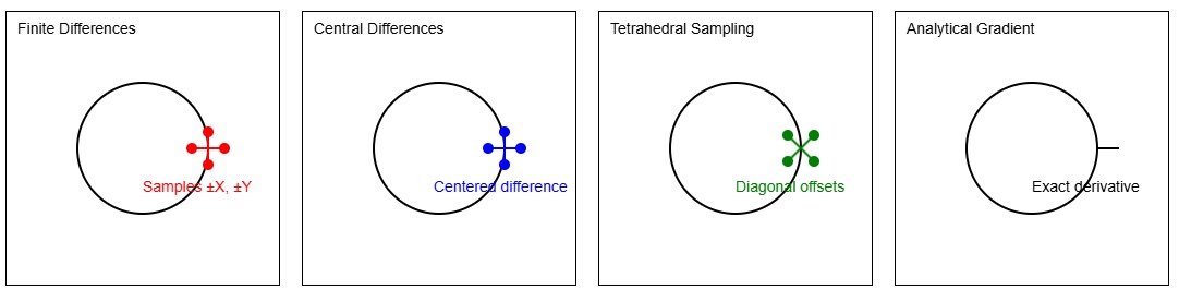
SDF Normal Estimation Comparison - Visualizing different methods with labeled diagrams.
This is easy - however, the old saying goes 'there is more than one way to skin a cat' - as with calculating the normal - there are lots of ways of doing this. Each having pros and cons.
Table comparing different methods for calculating normals for Signed Distance Functions (SDFs), focusing on their advantages and trade-offs:
Method
Description
Pros
Cons
Finite Differences
Computes normals by taking differences along axis-aligned directions.
Simple and easy to implement Works with any SDF function
equires 6 samples per evaluation Can produce small artifacts due to numerical precision
Tetrahedral Sampling
Uses four predefined directional vectors to estimate the gradient.
Fewer samples (4 instead of 6) Less axis-aligned bias Slightly more stable in some cases
Can introduce slight asymmetry Less intuitive compared to finite differences
Analytical Gradient
Uses symbolic differentiation or known gradient formulas for specific SDFs.
Exact normals No numerical approximation needed More efficient when available
Requires explicit gradient expressions Not always available for complex or composite SDFs
Central Differences
A variation of finite differences using a centered approach.
More accurate compared to forward/backward difference Fewer artifacts than simple finite difference
Requires 6 samples Still subject to precision issues
Dual Number Gradient
Uses automatic differentiation through dual numbers to compute exact gradients.
Precise for analytical functions Efficient in certain cases
Harder to implement for general SDFs Requires specialized math handling
There are many other ones - including Sobel-like Sampling (for stylization or extra robustness) and Stochastic Normal Estimation (Monte Carlo-style gradient).
Each method has trade-offs between precision, performance, and ease of implementation. If you're working on ray marching or procedural rendering, the choice depends on your optimization needs!
Theory To Working Implementations
We'll implement a simple WGSL function for the different normal calculation methods using Signed Distance Functions (SDFs).
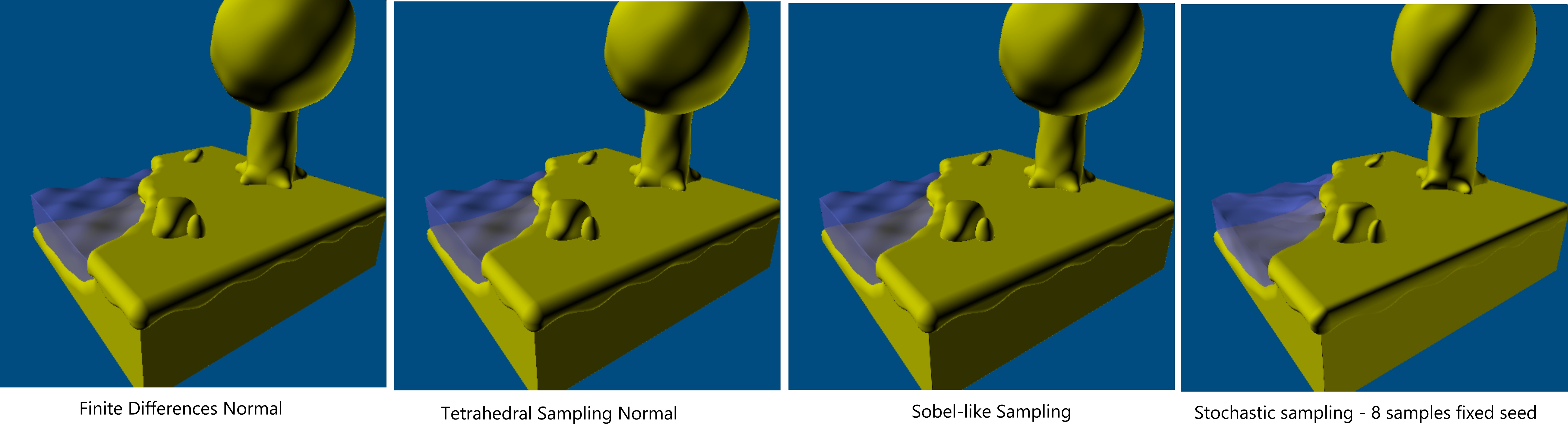
Screenshots from our test scene for the different normal calculations. The implementation algorithms are given below and the test code is included at the bottom (WebGPU Lab).
What To Look For?
When looking at the generated output for the scene using the different normal algorithms - you should look for key differences in shading, smoothness, and edge definition. Finite Differences often produce a subtle graininess or minor artifacts due to numerical precision, especially on curved surfaces. Central Differences may yield slightly more stable shading but can still show sampling-related inconsistencies. Tetrahedral Sampling tends to avoid axis-aligned bias, resulting in smoother gradients, but might introduce asymmetries in certain areas. Pay close attention to how light interacts with the surface—are highlights correctly positioned, do shadows behave naturally, and is there any visible noise or distortion at sharp transitions? These comparisons will help you evaluate which method best suits your needs in terms of quality versus performance trade-offs.
1. Finite Differences Normal
This method samples the SDF at small offsets along the x, y, and z axes.
• Slightly more accurate than finite differences
• Still requires 6 samples
5. Dual Number Gradient (Automatic Differentiation)
This method uses specialized algebra to get exact gradients. WGSL does not natively support dual numbers, but we can implement helper functions to manage the mathematics.
Implementing a normal function for an SDF (signed distance function) using dual numbers in WGSL (WebGPU Shading Language) allows you to compute exact gradients via automatic differentiation. This is especially valuable when analytical gradients are difficult or cumbersome to derive.
We compute the normal at a point on a surface defined by an SDF
map(p: vec3<f32>) -> f32
, using dual numbers for gradient estimation.
Background on Dual Numbers
A dual number is of the form:
<?php
a + bε, where ε^2 = 0 and ε ≠ 0
For a function
f(x + ε) = f(x) + f'(x)ε
, it lets us extract derivatives automatically.
We simulate dual numbers by creating a struct that carries a value and its partial derivatives (dx, dy, dz). Each arithmetic operation must propagate these components correctly.
Step-by-step Details Dual-Number Implementation
1. Define a
Dual3
struct representing a 3D dual number.
2. Overload math functions to operate on
Dual3
.
3. Define
map_dual
that takes
Dual3
and returns a dual number representing the SDF value and gradient.
4. Extract the gradient to get the normal.
• Accurate gradients even for complex analytic SDFs.
• No need for finite difference hacks or tuning epsilon.
• Can be generalized to more complex SDF trees.