A perceptron is a single layer neural network and a multi-layer perceptron is called Neural Networks. Think of a perceptron as a brick and a wall (collection of bricks) is a neural network.
The perceptron is a very simple component - if you understand how a perceptron works, the you should be able to master how a neural network works! Built on the same concept.
Single Perceptron
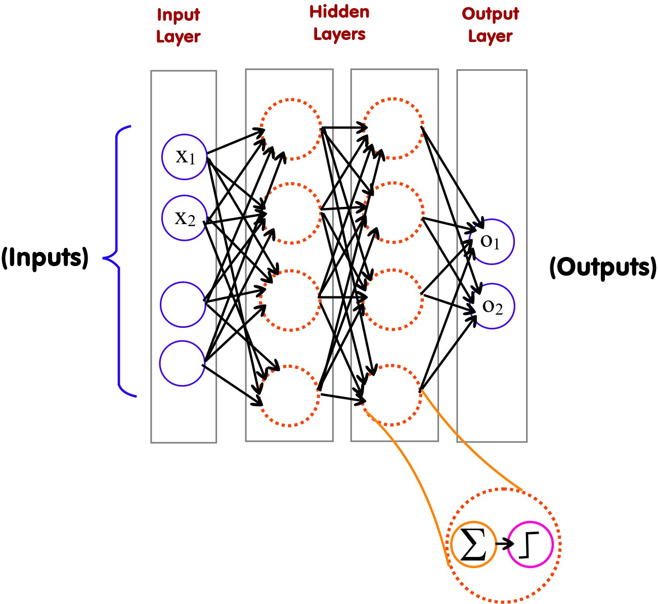
Connect More Perceptrons (Layers)
As you connect more and more perceptrons together in layers this is where the magic starts to happen. A single perceptron is limited in what it's able to accomplish (simple binary classification). Lots of perceptrons (neural network) is akin to a brain - and is able to simulate complex models.
Before jumping into neural networks (and deep neural networks - networks with lots and lots of layers) - let's look at a perceptron in detail.
Neural Networks and perceptrons are built on the same principles (work the same way). So, if you want to know how neural network works, learn how perceptron works.
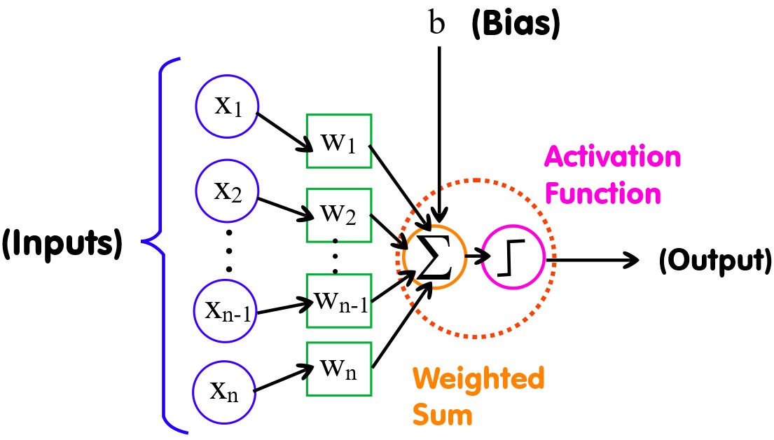
A perceptron consists of 4 parts:
1. Input values
2. Weights and Bias
3. Net sum
4. Activation Function
The equation for the perceptron is given by:
\[ y = \phi(\mathbf{w} \cdot \mathbf{x} + b) \]
where:
- \(\mathbf{w} = [w_1, w_2, \ldots, w_n]\) is the weight vector.
- \(\mathbf{x} = [x_1, x_2, \ldots, x_n]\) is the input vector.
- \(b\) is the bias term.
- \(\cdot\) represents the dot product.
- \(\phi\) is the activation function (this depends on the type of logic you're aiming to )
The perceptron outputs a decision based on the weighted sum of its inputs plus the bias which is passed through an activation function.
The activation function is a simple mathematical function that determines the output of a neuron given its inputs and weights.
It is crucial for introducing non-linearity into the model, enabling the network to learn complex patterns and decision boundaries.
Without the activation function, the neuron is simply a 'linear equation' - sums up the inputs which are multiplied by a scale. Which is fine, but is very limited.
An activation function can be something as simple as a threshold step (if the value is greater than some value it's 1 otherwise it's 0).
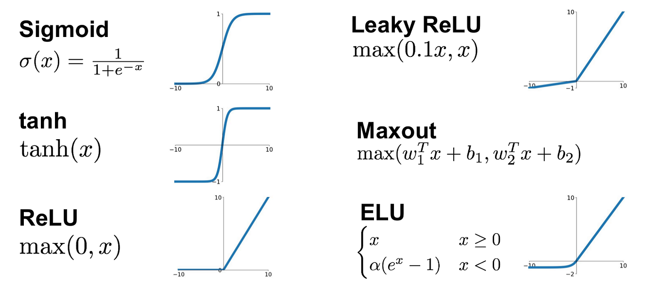
There are a variety of activation functions, such as the sigmoid function, hyperbolic tangent (tanh), and rectified linear unit (ReLU).
Each type of activation function has unique properties that make it suitable for different tasks: sigmoid and tanh functions are smooth and have outputs ranging between specific bounds, making them useful for probabilistic interpretations, while ReLU introduces sparsity and efficient gradient propagation, making it popular for deep learning.
As you'll learn, which activation function you choose can significantly impacts the learning capabilities and performance of your neural network.
Activation Functions
At this point it's worth providing a table so you can see the equations for the most popular activiation functions.
| **Activation Function** | **Equation**                       | **Details**                                                                                                                                      | **When to Use / Limits**                                                                                                         |
|-------------------------|------------------------------------|--------------------------------------------------------------------------------------------------------------------------------------------------|----------------------------------------------------------------------------------------------------------------------------------|
| **Step Function**       | \(\phi(z) = \begin{cases} 1 & \text{if } z \ge 0 \\ 0 & \text{if } z < 0 \end{cases}\) | Simple threshold function that outputs binary values.                                                                                            | Use in simple binary classifiers (e.g., perceptrons). Limited in complex tasks due to lack of smooth gradients for learning.     |
| **Sigmoid**             | \(\sigma(z) = \frac{1}{1 + e^{-z}}\) | Smooth, differentiable function outputting values between 0 and 1.                                                                                | Good for binary classification and probabilistic interpretations. Can suffer from vanishing gradients.                           |
| **Tanh**                | \(\tanh(z) = \frac{e^z - e^{-z}}{e^z + e^{-z}}\) | Smooth, differentiable function outputting values between -1 and 1.                                                                                | Useful in hidden layers for zero-centered outputs. Also can suffer from vanishing gradients, though less than sigmoid.           |
| **ReLU**                | \(\text{ReLU}(z) = \max(0, z)\)      | Outputs zero for negative inputs and linear for positive inputs, introducing sparsity and efficient computation.                                   | Common in hidden layers of deep networks. Can suffer from dying ReLU problem where neurons get stuck during training.            |
| **Leaky ReLU**          | \(\text{Leaky ReLU}(z) = \begin{cases} z & \text{if } z \ge 0 \\ \alpha z & \text{if } z < 0 \end{cases}\) | Modified ReLU allowing small negative values for negative inputs with \(\alpha\) being a small constant.                                          | Mitigates dying ReLU problem, making it suitable for deep networks. \(\alpha\) typically set to 0.01.                           |
| **Parametric ReLU (PReLU)** | \(\text{PReLU}(z) = \begin{cases} z & \text{if } z \ge 0 \\ \alpha z & \text{if } z < 0 \end{cases}\) | Similar to Leaky ReLU but \(\alpha\) is learned during training.                                                                                   | Offers flexibility over Leaky ReLU. Can potentially adapt better during training.                                               |
| **Softmax**             | \(\text{Softmax}(z_i) = \frac{e^{z_i}}{\sum_{j} e^{z_j}}\) | Converts a vector of values into a probability distribution.                                                                                       | Ideal for the output layer of multi-class classification problems. Ensures output probabilities sum to 1.                       |
| **ELU (Exponential Linear Unit)** | \(\text{ELU}(z) = \begin{cases} z & \text{if } z \ge 0 \\ \alpha (e^z - 1) & \text{if } z < 0 \end{cases}\) | Like ReLU but smooth for negative inputs, reducing bias shift and encouraging more effective learning.                                           | Suitable for deep networks. Requires more computation compared to ReLU. Parameter \(\alpha\) typically set to 1.                |
The table is a lot to take in at this point, but it summarizes the key aspects of popular activation functions (understanding their equations, characteristics, and practical applications).
Visualizating the shape of activation functions.
Important Points
• Weights shows the strength of the particular node.
• A bias value allows you to shift the activation function curve up or down.
• An activation functions is used to map the input between the required values like (0, 1) or (-1, 1).
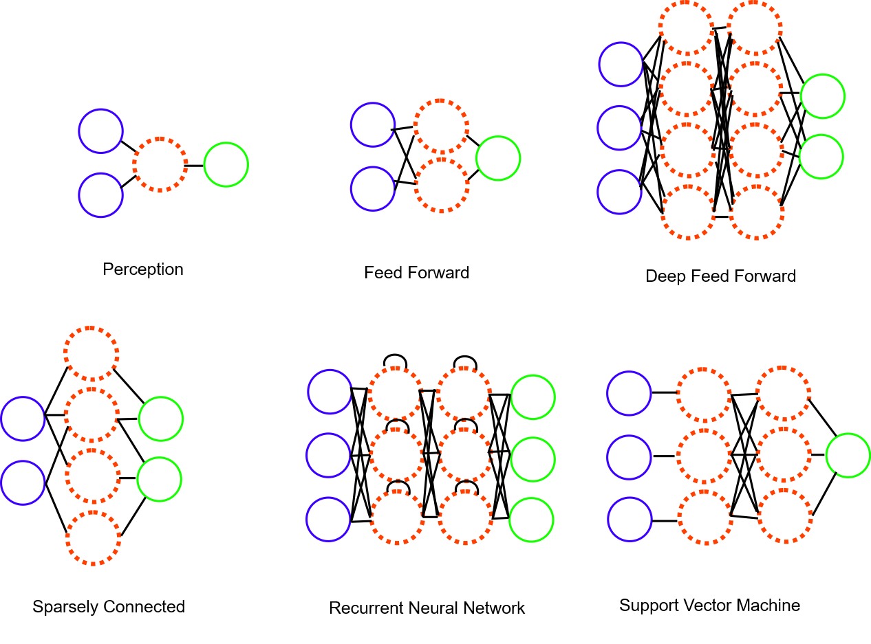
Network configurations
Connecting perceptrons together allows us to construct neural networks. As you can imagine there are lots of different ways of connecting neural networks (i.e., neural network topology shapes).
Full collected feed forward neural network (4:4:4:2)
Feed Forward Networks
A Feed Forward Network is a type of artificial neural network where connections between the nodes do not form a cycle, and data flows strictly from input to output layers through one or more hidden layers. A Deep Feed Forward Network extends this concept by having multiple hidden layers, allowing it to model more complex functions and patterns in the data.
Visual illustration of some neural network shapes (topologies).
Common feedforward topology shapes, include:
1. Fully Connected (Dense) Networks:
- Each neuron in one layer is connected to every neuron in the subsequent layer. This is the standard topology for most neural networks.
2. Convolutional Neural Networks (CNNs):
- Designed for processing structured grid data like images, CNNs use convolutional layers, pooling layers, and fully connected layers. They are typically arranged in a hierarchical structure with convolutional and pooling layers followed by one or more dense layers.
3. Recurrent Neural Networks (RNNs):
- Though primarily used for sequential data, they can be part of a feedforward network when unrolled. Each time step can be viewed as a layer in a deep feedforward network.
4. Residual Networks (ResNets):
- Use skip connections (or shortcuts) to jump over some layers. This helps in mitigating the vanishing gradient problem and allows the training of very deep networks.
5. Inception Networks:
- Utilize parallel convolutional layers with different kernel sizes at each layer level. The outputs of these convolutions are concatenated and passed to the next layer.
6. U-Net:
- Typically used for image segmentation, it has a symmetric architecture with an encoder (contracting path) and a decoder (expanding path), with skip connections between layers of the same level in the encoder and decoder.
7. Autoencoders:
- Consist of an encoder and a decoder. The encoder compresses the input into a latent space representation, and the decoder reconstructs the input from this representation.
8. Multilayer Perceptron (MLP):
- The simplest form of feedforward neural network, where each layer is fully connected, and all nodes in one layer connect to all nodes in the next layer.
9. Sparse Networks:
- Similar to fully connected networks but with some connections removed according to a predefined sparsity pattern, which can reduce the number of parameters and computation.
10. Capsule Networks:
- Use groups of neurons (capsules) to represent different properties of an object part and their spatial relationships. Capsule layers can be seen as more complex feedforward layers.
Remember, you're not limited to these topologies. Once you understand how to implement a neural network you can connect them together however you want to suit specific applications and to improve performance, efficiency, and accuracy.
Be careful with non-conventional (bespoke) neural network configurations/shapes/topologies - it can turn into a mess to manage and train.
Networks Shape
The shape and structure of a neural network can impact its suitability for massively parallel architectures (like the GPU). As you can see, the perceptrons are connected together by links - which introduces 'data dependancies'. Ideally, for the GPU to be as efficient as possible (so we can get the massive speedup we are looking for), we want to make the neural network as 'parallel' as possible. That is, we want to be able to perform as many parallel computations as possible at the same time.
For example, feed forward networks can be represented as layers and matrix blocks which store the weight and bias coefficients - and the GPU likes matrices.
Training & Data
Neural networks use supervised learning to configure the coefficients (weights and biases) to perform a specific task. This means, they need data! Data to train the neural network.
This data usually comes in the form on example input and output values - which the neural network tries to connect (model the relationship). So for any input it is able to predict the output (even for inputs it has never seen before).
Train the neural network to learn the patterns fo the data (reproduces the same result given the data but also is able to generate result that correlate with the dataset characteristics if the input is not the same as one of the inputs from the dataset). A simple example of this, would be a sine wave - if you give it enough sample points it should know that the output is a sine wave - so for any input the output will be on the sine wave output.
Order of the data - random - if it's sequential and always in the same order - the neural network will expect the real-world data to always be in the same order! It expects and learns the patterns you give it (including the order of the data).
Training Backpropogation
There are lots of different ways of training neural networks. However, one of the most popular is backpropogation; which uses error gradient to correct the weights and biases. Backpropogation has the advantage of being efficient and fast; and can be ported to parallel architectures (like the GPU).
The steps for the backpropgation training are an iterative process that does a forward pass to get the output and compares this with the ideal value. Using this is calculates the gradients for each layer - making small corrections to the weights and biases.
Remember, for the feedforward we calculate the activations of each layer sequentially starting from the input layer. For an input vector \(X\), the activation \(Z_1\) of the first hidden layer is calculated as \(Z_1 = W_1 \cdot X + b_1\), where \(W_1\) and \(b_1\) are the weights and biases for the hidden layer, respectively. These activations are then passed through a sigmoid activation function to produce the output of the hidden layer: \(A_1 = \sigma(Z_1)\), where \(\sigma(x) = \frac{1}{1 + e^{-x}}\). This process is repeated for the output layer, where the activations \(Z_2\) are calculated as \(Z_2 = W_2 \cdot A_1 + b_2\), and the final output is obtained as \(A_2 = \sigma(Z_2)\).
While the backpropagation involves computing the gradients of the loss function with respect to the network's weights and biases, starting from the output layer and moving backward. For the output layer, the error \(\delta_2\) is calculated as \(\delta_2 = (A_2 - Y) \cdot \sigma'(Z_2)\), where \(Y\) is the target output, and \(\sigma'(Z_2)\) is the derivative of the sigmoid function. For the hidden layer, the error \(\delta_1\) is computed as \(\delta_1 = (W_2^T \cdot \delta_2) \cdot \sigma'(Z_1)\). The weights and biases are then updated using the calculated gradients and the learning rate \(\eta\): \(W_2 = W_2 - \eta \cdot \delta_2 \cdot A_1^T\) and \(b_2 = b_2 - \eta \cdot \delta_2\) for the output layer, and similarly \(W_1 = W_1 - \eta \cdot \delta_1 \cdot X^T\) and \(b_1 = b_1 - \eta \cdot \delta_1\) for the hidden layer.
Backprogation Steps
1. Initialize weights (\(W_1, W_2\)) and biases (\(b_1, b_2\)). 2. Perform forward pass to calculate activations:
- Compute \(Z_1 = W_1 \cdot X + b_1\).
- Apply activation function \(A_1 = \sigma(Z_1)\).
- Compute \(Z_2 = W_2 \cdot A_1 + b_2\).
- Apply activation function \(A_2 = \sigma(Z_2)\).
3. Compute the loss using the predicted output \(A_2\) and actual target \(Y\).
7. Repeat steps 2-6 for a number of epochs or until convergence.
These pseudo steps outline the backpropagation process, detailing the calculation of gradients and the subsequent update of weights and biases. The process iteratively adjusts the model parameters to minimize the loss, thereby training the neural network.
XOR Test Case
Instead of just picking random values for the input and output (which you can) - a popular test case for neural networks is the XOR logic gate (classic benchmark in the field of neural networks).
The XOR problem, despite its simplicity, encapsulates the essence of what makes neural networks powerful: their ability to model complex, non-linear relationships. Its role in the history of neural network research underscores the importance of multi-layer architectures and continues to be a fundamental teaching and testing tool in the field.
Why an XOR?
• Simple binary classification problem
• Easy to understand (mathematics are easy) - binary inputs (0 or 1) and produces a binary output (0 or 1)
• Not linearly separable (i.e., cannot draw a single straight line to separate the classes in the input space)
In fact, early neural network like the single-layer perceptron failed to solve the XOR problem - highlighting the limitations of simple linear models (and why we need the activiation function).
An XOR problem needs one or more hidden layers, which allow you to test the model's non-linear decision boundaries.
One of the 'hello world' test cases - its historical significance has made the XOR problem one of the first test cases (especially in educational settings). It serves as a minimal example that requires a multi-layer network to be solved, thereby helping students and newcomers understand the necessity and functionality of deeper networks.
Just incase you're never stumbpled across XOR logic, the XOR truth table for a 2 input 1 output is:
This table shows that the XOR function outputs true (1) when the inputs are different and false (0) when they are the same.
Better Backpropagation
Improving backpropagation to ensure faster and more reliable convergence involves various techniques that can be applied to the neural network training process.
As the WebGPU model evolves you can expand the backpropagation approach by combining techniques to get better convergence during neural network training.
The list of engineering fixes are not a one size fits all - their combination and tuning might depend on the particular problem and dataset you are working with.
• 1. Learning Rate Adjustment
- Adaptive Learning Rates: Use algorithms like AdaGrad, RMSprop, or Adam, which adjust the learning rate during training.
- Learning Rate Scheduling: Reduce the learning rate as training progresses, which helps to fine-tune the weights as the algorithm approaches the minimum.
• 2. Weight Initialization
- Xavier Initialization: Suitable for sigmoid and tanh activation functions.
- He Initialization: Suitable for ReLU and its variants.
Proper weight initialization can prevent gradients from vanishing or exploding, facilitating smoother training.
• 3. Gradient Clipping
- Clip Gradients: This technique involves limiting the gradients to a maximum value to prevent exploding gradients, especially in recurrent neural networks.
• 4. Regularization Techniques
- L2 Regularization: Also known as weight decay, it helps in reducing overfitting by penalizing large weights.
- Dropout: Randomly turning off a subset of neurons during training to prevent overfitting.
- Batch Normalization: Normalizes the inputs of each layer, which helps in stabilizing and accelerating the training process.
• 5. Optimizers
- Momentum: Helps accelerate gradients vectors in the right directions, leading to faster converging.
- Nesterov Accelerated Gradient (NAG): A variant of momentum that looks ahead to improve the update.
• 6. Mini-Batch Gradient Descent
Using mini-batches rather than the entire dataset or a single example helps to balance the convergence speed and stability.
• 7. Activation Functions
- ReLU and its Variants: Use activation functions like Leaky ReLU, Parametric ReLU, or Exponential Linear Units (ELU) that mitigate the vanishing gradient problem.
- Swish or Mish: More recent activation functions that sometimes outperform traditional functions like ReLU.
• 8. Loss Function Engineering
Choosing an appropriate loss function or engineering it to suit the problem can also impact the convergence. For example, using cross-entropy loss for classification problems rather than mean squared error.
• 9. Data Preprocessing
- Normalization: Normalize the input data to have zero mean and unit variance.
- Data Augmentation: Use techniques like rotation, flipping, scaling, etc., to artificially increase the size and variability of the training set.
• 10. Early Stopping
Monitor the model's performance on a validation set and stop training when the performance stops improving to avoid overfitting.
• 11. Learning Rate Warm-up
Start with a lower learning rate at the beginning of the training and gradually increase it to the desired value.
• 12. Cyclical Learning Rates
Alternate between higher and lower learning rates in a cyclical fashion, which can help escape local minima and saddle points.
Visitor:
Copyright (c) 2002-2026 xbdev.net - All rights reserved.
Designated articles, tutorials and software are the property of their respective owners.