www.xbdev.net
xbdev - software development
Friday February 6, 2026
Home | Contact | Support | WebGPU Graphics and Compute ... | Neural Networks and WebGPU Compute.. Learning from Data.....


Neural Networks and WebGPU Compute..

Learning from Data.....


Visualizing Neural Networks


Very simple to draw the neural nework data visually on screen - all the inputs/ouputs/nodes/weight and more - you can even update this data on the fly to show how the neural network is evolving (during training).

For low-dimensional neural networks you can use nodes and connections - for high-density cases (e.g., thousands or millions of nodes - you'll probably display the neural network data as a color image - colors indicating number ranges).


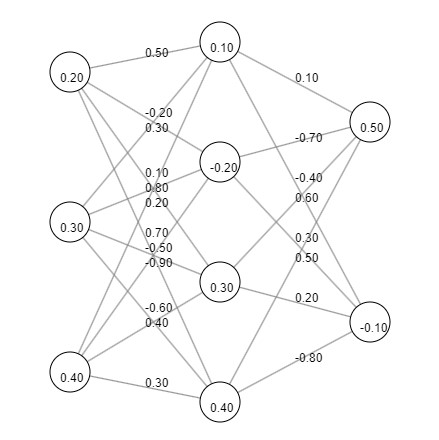
Neural network visualiztion (connections, layers, weights and biases).


If you're going to visualize the network data in real-time (during training) - avoid doing it every frame - instead only do it every so often - so it only updates every few seconds. You can use a counter and a modulus to triger the update in code (such as, update every 100 iterations in code:
count%100==
)


Visualizing Network Connections


Complete Code


/*
Neural Network Visualization

Inputs on the left and the outputs on the right - in between are all the hidden nodes/connections.
For fully connected neural networks.
*/

// Write a function that does all the work! A single function - just pass the neural network configuration data and it'll create it (or update it if one already exists).


function drawNeuralNetwork(canvasNameconfig) {
let canvas document.getElementById(canvasName);
if ( 
canvas==undefined )
{
    
canvas document.createElement('canvas');
    
document.body.appendChildcanvas );
    
canvas.width canvas.height 600;
}
const 
context canvas.getContext('2d');
const 
canvasWidth  context.canvas.width;
const 
canvasHeight context.canvas.height;

const { 
layersweightsbiases } = config;

const 
layerCount layers.length;
const 
neuronRadius 20;
const 
layerSpacing canvasWidth / (layerCount 1);
const 
maxNeurons Math.max(...layers);

// Function to get position of a neuron
function getNeuronPosition(layerIndexneuronIndex) {
  const 
layerSpacing * (layerIndex 1);
  const 
ySpacing canvasHeight / (layers[layerIndex] + 1);
  const 
ySpacing * (neuronIndex 1);
  return { 
x};
}

// Draw connections, weights and biases
for (let i 0layerCount 1i++) {
  for (
let j 0layers[i]; j++) {
  for (
let k 0layers[1]; k++) {
    const 
from getNeuronPosition(ij);
    const 
to getNeuronPosition(1k);
    
context.beginPath();
    
context.moveTo(from.xfrom.y);
    
context.lineTo(to.xto.y);
    
context.strokeStyle 'gray';
    
context.stroke();

    
// Draw weight value
    
const weight weights[i][j][k];
    const 
midX = (from.to.x) / 2;
    const 
midY = (from.to.y) / 2;
    
context.fillStyle 'black';
    
context.font '12px Arial';
    
context.fillText(weight.toFixed(2), midXmidY);
  }
  }
}

// Draw neurons and biases
for (let i 0layerCounti++) {
  for (
let j 0layers[i]; j++) {
  const { 
x} = getNeuronPosition(ij);

  
// Draw neuron
  
context.beginPath();
  
context.arc(xyneuronRadius0Math.PI);
  
context.fillStyle 'white';
  
context.fill();
  
context.strokeStyle 'black';
  
context.stroke();

  
// Draw bias
  
const bias biases[i][j];
  
context.fillStyle 'black';
  
context.font '12px Arial';
  
context.fillText(bias.toFixed(2), neuronRadius 2neuronRadius 2);
  }
}
}
// drawNeuralNetwork


// Example configuration
const config = {
layers: [342], // Number of neurons per layer (input layer, hidden layers, output layer)
weights: [
  
// Weights between layer 0 and layer 1
  
[
    [
0.5, -0.20.10.7], // Weights from neuron 0 in layer 0 to neurons in layer 1
    
[0.30.8, -0.5, -0.6],
    [
0.2, -0.90.40.3]
  ],
  
// Weights between layer 1 and layer 2
  
[
    [
0.1, -0.4], // Weights from neuron 0 in layer 1 to neurons in layer 2
    
[-0.70.3],
    [
0.60.2],
    [
0.5, -0.8]
  ]
],
biases: [
  
// Biases for layer 0
  
[0.20.30.4],
  
// Biases for layer 1
  
[0.1, -0.20.30.4],
  
// Biases for layer 2
  
[0.5, -0.1]
]
};

drawNeuralNetwork('neuralNetworkCanvas'config);


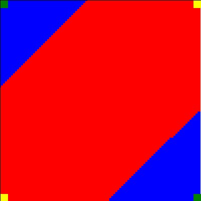
Plotting the Input vs Output


We can visualize the neural network's sensitivity to the input and output. Plotting the outputs in a grid of input values, we can visually inspect the decision boundary created by the neural network.

Red and blue colors represent the network's prediction for each point in the input space, making it easy to see how well the network distinguishes between the two classes (output
0
and
1
).

The green dots indicate the original training points, allowing us to assess the accuracy of the neural network's learning. This visualization helps to understand the network's performance and the effectiveness of its training in solving a non-linear classification problem.


Output when plotting the input vs the output for trained neural network (XOR).


For the example, we'll use of the open source JavaScript libraries called 'Synaptic'.


Neural Networks and Deep Learning with Javascript (Examples/Hands-On Approach)

Learn about neural networks and deep learning architechtures from the ground-up. Not just the mathematics - but actually getting simple neural networks up and running that perform a variety of cool things - from learning your web-cam to control a video game, analysis images or identify patterns in data.


This example demonstrates the XOR problem visually, showing how the neural network separates the input space into different output regions.

<h1>Neural Network XOR Plot</h1>

<
canvas id="canvas" width="400" height="400"></canvas>
<
script src="https://cdnjs.cloudflare.com/ajax/libs/synaptic/1.1.4/synaptic.js"></script>

<
script>
    
// Create the neural network
    
const { LayerNetworkTrainer } = synaptic;

    const 
inputLayer  = new Layer(2);
    const 
hiddenLayer = new Layer(3);
    const 
outputLayer = new Layer(1);

    
inputLayer.project(hiddenLayer);
    
hiddenLayer.project(outputLayer);

    const 
myNetwork = new Network({
        
inputinputLayer,
        
hidden: [hiddenLayer],
        
outputoutputLayer
    
});

    
// XOR training set
    
const trainingSet = [
        { 
input: [00], output: [0] },
        { 
input: [01], output: [1] },
        { 
input: [10], output: [1] },
        { 
input: [11], output: [0] }
    ];

    
// Train the neural network
    
const trainer = new Trainer(myNetwork);
    
trainer.train(trainingSet, {
        
rate0.2,
        
iterations20000,
        
error0.005,
        
shuffletrue,
        
log1000,
        
costTrainer.cost.CROSS_ENTROPY
    
});

    
// Plotting function
    
const canvas document.getElementById('canvas');
    const 
ctx canvas.getContext('2d');

    function 
plotPoint(xycolorw=6h=6) {
        
ctx.fillStyle color;
        
ctx.fillRect(400 w*0.5400 w*0.5wh);
    }

    
// Generate points and plot
    
for (let i 0<= 1+= 0.01) {
        for (
let j 0<= 1+= 0.01) {
            const 
output myNetwork.activate([ij]);
            const 
color output[0] > 0.5 'red' 'blue';
            
plotPoint(ijcolor);
        }
    }

    
// Plot original data points
    
plotPoint(00'green' 3030);
    
plotPoint(01'yellow'3030);
    
plotPoint(10'yellow'3030);
    
plotPoint(11'green' 3030);
</
script>


Things to Try


• Make the connecting lines reflect the weight magnitude (thicker or thiner lines)
• Draw the activation function type on the visual (e.g., signmoid or relu)
• Interaction - cursor hovers over a node or link it changes color/emphasised (show extra information)
• Color information for magnitude or numerical ranges (0-1 maps to red-green-blue range)
• Incorporating shapes to provide context
• Draw a line from the input to the output - emphasis the strongest influence using the largest weight from each layer to decide the path
• Add tables for the data that can be sorted high/low (with color cells) - 0 to 1 (mapping to blue to red)


Resources and Links


• Neural Network Visualization Code [LINK]

• Graph In vs Oupt (Notebook) [LINK]


WebGPU by Example: Fractals, Image Effects, Ray-Tracing, Procedural Geometry, 2D/3D, Particles, Simulations WebGPU Compute graphics and animations using the webgpu api 12 week course kenwright learn webgpu api kenwright programming compute and graphics applications with html5 and webgpu api kenwright real-time 3d graphics with webgpu kenwright webgpu api develompent a quick start guide kenwright webgpu by example 2022 kenwright webgpu gems kenwright webgpu interactive compute and graphics visualization cookbook kenwright wgsl webgpu shading language cookbook kenwright wgsl webgpugems shading language cookbook kenwright


Advert (Support Website)

 
 Visitor:
Copyright (c) 2002-2025 xbdev.net - All rights reserved.
Designated articles, tutorials and software are the property of their respective owners.