Ray-tracing is so much more ... there are all sorts of flavors with different features. Ray-tracing is often termed as the overhanging technique where rays are cast from the eye into the scene, tracing their interactions with objects to calculate color, reflection, and refraction. It forms the basis of most advanced rendering techniques.
However, the calculations for the rays, their interactions and components let us seperate ray-tracing into various models/categories.
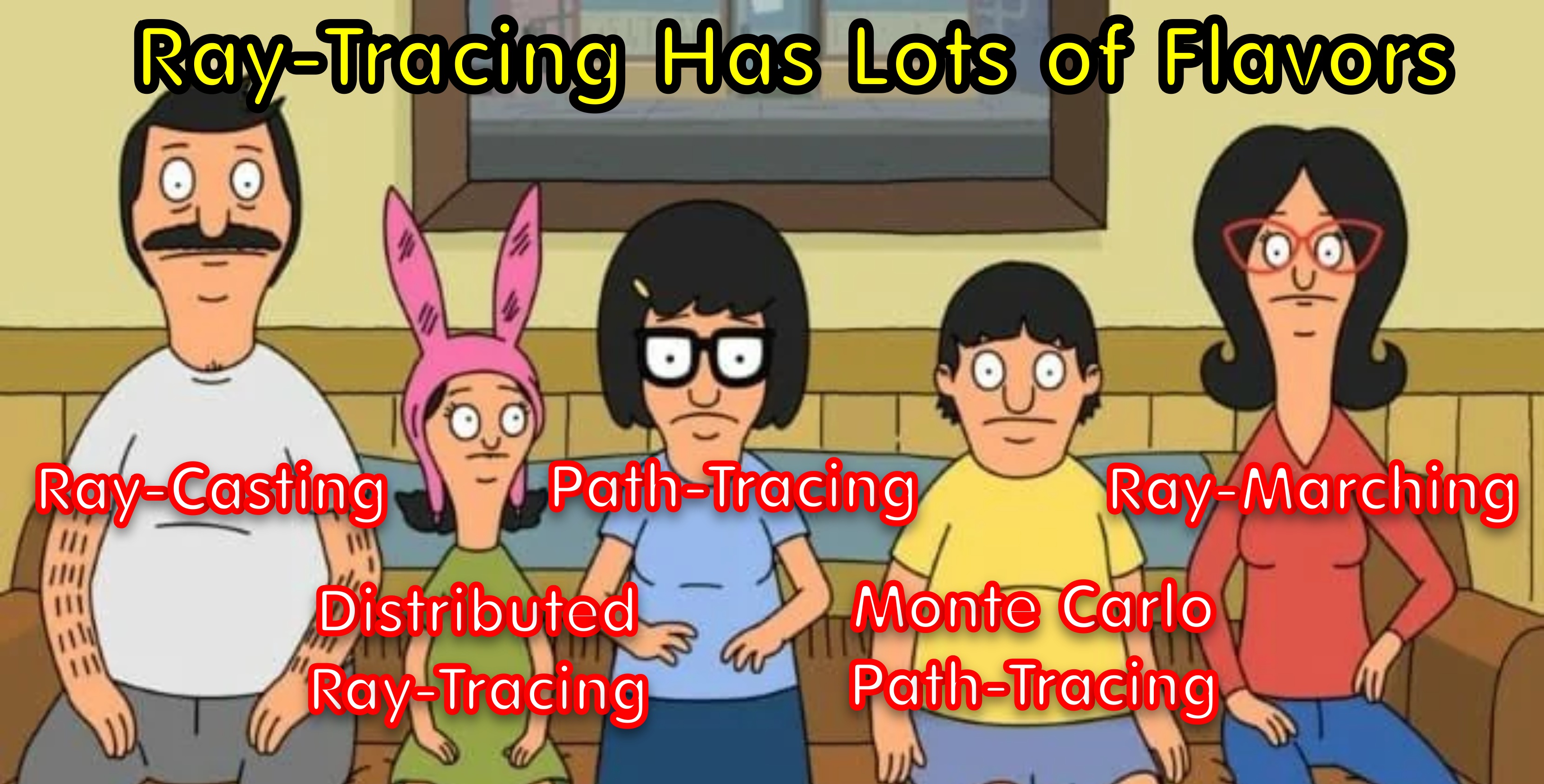
Ray-tracing is like a rabbit-hole - more complex than you thought! As Bob learned from Bob's Burgers (s11e02) - when he goes online to do some research and when he comes back he's shocked - and says - "Okay, uh, I-I saw some things, um... I am not the same person I used to be..". Unlock your mind to the broader ray-tracing fundamentals. You won't be the same!
Overview of Fundamentals
Grouping ray-tracing techniques highlights their shared foundational principles, such as simulating the behavior of light through rays, while distinguishing their unique focuses, like handling explicit geometry, volumetrics, or procedural content. It showcases the evolution from simple models like ray casting to complex hybrids, reflecting the trade-offs between realism, performance, and flexibility.
Grouping
Concept
Description
Related Techniques
Foundational Principles
Backward Ray Tracing
Traces rays from the camera to the scene.
Path Tracing, Whitted Ray Tracing.
Forward Ray Tracing
Traces rays from light sources to the scene.
Photon Mapping, Bidirectional Path Tracing.
Recursive Tracing
Rays are traced recursively (e.g., reflections/refractions).
Whitted Ray Tracing, Bidirectional Tracing.
Energy Transport Models
Monte Carlo Sampling
Uses randomness for solving the rendering equation.
Path Tracing, MLT, Progressive Photon Mapping.
Radiance Transfer
Simulates energy transfer between surfaces or volumes.
Radiosity, Ray Marching.
Efficiency Techniques
Importance Sampling
Focuses on sampling areas of high contribution.
Monte Carlo, MLT.
Hierarchical Subdivision
Dynamically refines geometry or light transfer areas.
Hierarchical Radiosity, Adaptive Ray Marching.
Hierarchy of Models/Techniques
Viewing the hierarchy of ray-tracing models and techniques provides a clear understanding of how different methods are related, highlighting their unique purposes and overlaps. It enables developers to choose the most suitable approach for specific applications, from realistic rendering to real-time effects, based on trade-offs like computational cost and visual fidelity. Additionally, it fosters a deeper appreciation of hybrid techniques, which combine strengths from multiple methods for optimal performance and quality.
Ray Tracing
├── Ray-Casting
├── Recursive Ray Tracing
├── Whitted-Style Ray Tracing
├── Distributed Ray Tracing
├── Path Tracing
├── Unidirectional Path Tracing
├── Bidirectional Path Tracing
├── Progressive Path Tracing
├── Stochastic Path Tracing
├── Spectral Path Tracing
├── Volumetric Path Tracing
├── Monte Carlo Methods (general numerical approach)
├── Monte Carlo Path Tracing (specific Path Tracing subtype)
├── Metropolis Light Transport (MLT)
├── Ray Marching
├── SDF Ray Marching
├── Volumetric Ray Marching
├── Adaptive Ray Marching
├── Photon Mapping
├── Basic Photon Mapping
├── Progressive Photon Mapping
├── Stochastic Progressive Photon Mapping
├── Radiosity
├── Basic Radiosity
├── Hierarchical Radiosity
├── Hybrid Techniques
├── Voxel Cone Tracing
├── Ray Tracing + Rasterization
├── Path Space Metropolis Light Transport
Name
Sub-Techniques
Description
Key Features
Use Cases
Ray-Casting
None
A simple technique that casts rays from the camera to determine visibility of objects in the scene.
- Primary rays only
- No secondary effects like reflection or refraction
- Basic shading models
- Early 3D rendering
- Visibility determination
- Collision detection
Recursive Ray Tracing
- Whitted-Style Ray Tracing - Distributed Ray Tracing
Extends ray-casting by tracing secondary rays to simulate reflections, refractions, and shadows.
- Recursive handling of secondary rays
- Realistic reflections and refractions
- Shadows via shadow rays
- High-quality rendering
- Architectural visualization
- CGI for movies
A rendering method focused on simulating diffuse interreflections of light in a scene.
- Solves for light energy balance
- View-independent
- Suitable for static scenes
- Architectural pre-visualization
- Scene baking
- Accurate diffuse lighting
Hybrid Techniques
- Voxel Cone Tracing
- Ray Tracing + Rasterization
- Path Space Metropolis Light Transport
Combines ray tracing and rasterization to achieve a balance between performance and visual fidelity.
- Deferred or forward+ shading
- Uses rasterization for primary rays
- Ray tracing for reflections and shadows
- Real-time rendering
- Games with realistic effects
- Mixed media applications
Ray-Casting
Ray-Casting is a foundational rendering technique used in computer graphics where rays are cast from the camera (or viewer) into the scene to determine which objects are visible. It is often considered the simplest form of ray-based rendering and serves as the basis for more advanced techniques like ray tracing and path tracing.
Key Characteristics of Ray-Casting:
• Primary Rays Only • Ray-casting calculates intersections of rays with objects in the scene to determine visibility. It does not calculate secondary rays for effects like reflections, refractions, or shadows.
• Only simple shading models (e.g., Phong or Lambertian) are applied using direct illumination from light sources. No global illumination or indirect lighting is considered.
• Used in early 3D graphics applications like first-person shooter games (e.g., Wolfenstein 3D). Still used in certain areas like collision detection, picking objects in 3D editors, and visibility determination.
Recursive Ray Tracing
Recursive Ray Tracing is a broad model that handles recursive phenomena to simulate light transport with multiple bounces, typically for reflections, refractions, and shadows.
• How it works:
- Rays are recursively spawned when they interact with reflective or refractive surfaces.
- Each intersection generates one or more new rays (reflections or refractions) which are traced recursively until a stopping condition is met (e.g., a maximum number of bounces or negligible contribution).
• Advantages:
- Efficient for reflections, refractions, and shadows.
- Handles multiple bounces of light naturally, simulating realistic interactions with materials.
• Disadvantages:
- May not handle global illumination well without additional techniques.
- Can lead to excessive recursion, which requires careful termination and can result in artifacts like fireflies if not controlled properly.
Whitted Ray Tracing Whitted Ray Tracing is a subset of Recursive Ray Tracing. It uses recursion deterministically to model a small set of effects like reflections and refractions. Recursive Ray Tracing can extend beyond Whitted's model to include stochastic methods (Distributed Ray Tracing), global illumination (Path Tracing), or even volumetric effects (Ray Marching).
A specific implementation of Recursive Ray Tracing introduced by Turner Whitted in 1980. Whitted Ray Tracing is designed to simulate certain optical effects, such as:
• Perfect reflections (e.g., mirrors).
• Refractions (e.g., glass, water).
• Shadows (via shadow rays to light sources).
Key Characteristics Whitted Ray Tracing:
- Focuses on deterministic recursion.
- Each interaction generates a single reflected ray and/or single refracted ray.
- Often limited to primary effects like direct reflections and refractions without stochastic sampling.
- Output produces sharp, clean images with hard shadows, specular reflections, and refractions.
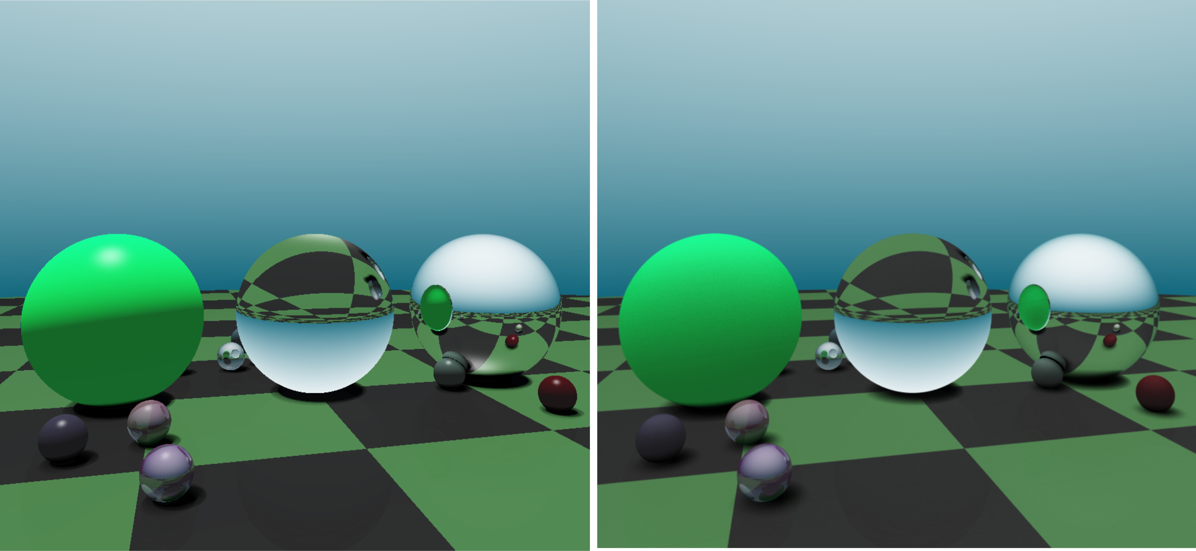
Distributed Ray Tracing (Stochastic Sampling)
Distributed Ray Tracing algorithm that generates multiple rays per pixel with slight variations to simulate effects like soft shadows, depth of field, and glossy reflections.
Introduce randomness through stochastic sampling to simulate natural light effects such as soft shadows, depth of field, motion blur, and light diffusion.
• How it works:
- For each primary ray, multiple rays are generated with slight variations in direction or origin.
- This sampling generates soft, blurry effects such as soft shadows or reflections that are averaged over several samples.
- Additional rays are used to simulate camera lens jitter for depth of field and motion blur for moving objects.
• Advantages:
- Simulates realistic natural effects like soft shadows, depth of field, and motion blur.
- Produces more photorealistic images than basic Whitted Ray Tracing.
• Disadvantages:
- Computationally expensive due to the large number of rays cast.
- Results in images with noise that require more samples to clean up.
- More complex to implement than Whitted Ray Tracing because of the stochastic nature.
Works by jittering the primary rays within each pixel.
Psuedo Code Example
Click to Show Details
function distributed_ray_tracing(scene, camera, image_width, image_height, samples_per_pixel):
    # Initialize an image buffer
    image = initialize_image(image_width, image_height)

    # Loop through each pixel in the image
    for y in range(image_height):
        for x in range(image_width):
            pixel_color = Vector3(0, 0, 0)  # Start with black
            for sample in range(samples_per_pixel):
                # Generate a primary ray with slight variations
                primary_ray = generate_primary_ray(camera, x, y, image_width, image_height)

                # Trace the ray through the scene and get its contribution
                sample_color = trace_ray(scene, primary_ray, 0)

                # Accumulate the color
                pixel_color += sample_color

            # Average the accumulated color for anti-aliasing
            pixel_color /= samples_per_pixel

            # Store the averaged color in the image buffer
            image[x, y] = pixel_color

    return image

# Function to generate a primary ray with distributed sampling
function generate_primary_ray(camera, x, y, image_width, image_height):
    # Add jitter for anti-aliasing
    jitter_x = random_float(-0.5, 0.5)
    jitter_y = random_float(-0.5, 0.5)
    pixel_x = x + jitter_x
    pixel_y = y + jitter_y

    # Adjust for depth of field
    lens_sample = sample_lens(camera.aperture_size)
    focus_point = calculate_focus_point(camera, pixel_x, pixel_y, lens_sample)

    # Generate ray from the camera through the pixel (with depth of field considerations)
    ray_origin = camera.position + lens_sample
    ray_direction = normalize(focus_point - ray_origin)

    return Ray(ray_origin, ray_direction)

# Recursive function to trace a ray through the scene
function trace_ray(scene, ray, depth):
    if depth > MAX_DEPTH:
        return Vector3(0, 0, 0)  # Return black if recursion limit is reached

    # Find the nearest intersection with the scene
    hit = scene_intersect(scene, ray)
    if not hit:
        return scene.background_color  # Return background color if no hit

    # Compute the direct lighting contribution
    surface_color = compute_direct_lighting(scene, ray, hit)

    # Handle reflections and refractions (if applicable)
    if hit.material.is_reflective:
        reflected_ray = compute_reflected_ray(ray, hit)
        surface_color += hit.material.reflectivity * trace_ray(scene, reflected_ray, depth + 1)

    if hit.material.is_refractive:
        refracted_ray = compute_refracted_ray(ray, hit)
        surface_color += hit.material.transparency * trace_ray(scene, refracted_ray, depth + 1)

    # Return the computed color
    return surface_color

# Function to compute direct lighting with soft shadows
function compute_direct_lighting(scene, ray, hit):
    total_light = Vector3(0, 0, 0)
    for light in scene.lights:
        shadow_ray = generate_shadow_ray(hit.position, light)
        if not scene_intersect(scene, shadow_ray):  # Light is not blocked
            light_contribution = calculate_light_contribution(light, hit)
            total_light += light_contribution
    return total_light

# Function to generate a shadow ray with distributed sampling (for soft shadows)
function generate_shadow_ray(surface_point, light):
    light_sample = sample_area_light(light)  # Random point on the area light
    return Ray(surface_point, normalize(light_sample - surface_point))
Path Tracing
Path tracing differs from traditional recursive ray tracing by incorporating randomness and statistical methods to simulate the many possible paths light can take in a scene. Instead of following a deterministic approach to trace rays for reflections, refractions, and shadows, path tracing uses Monte Carlo integration to sample indirect lighting paths, scattering rays at random directions according to material properties. This allows it to capture effects like global illumination, soft shadows, caustics, and diffuse interreflections, which are difficult or computationally infeasible in standard recursive ray tracing. While this results in more realistic images, it comes at the cost of requiring numerous samples per pixel to reduce noise.
Monte Carlo methods are a general numerical approach for solving problems using randomness and statistical sampling, applicable across various fields beyond rendering. While path tracing is one specific application of Monte Carlo techniques for light transport simulation in graphics, Monte Carlo encompasses a much broader range of algorithms, including importance sampling, stochastic integration, and Metropolis Light Transport, some of which extend beyond the scope of path tracing.
Monte Carlo Path Tracing
Monte Carlo Path Tracing is a global illumination algorithm that uses random sampling to simulate how light interacts with surfaces to produce photorealistic images. The algorithm handles complex lighting phenomena like indirect illumination, caustics, and soft shadows.
Pseudo-Code for Monte Carlo Path Tracing:
Click to Show Details
function monte_carlo_path_tracing(scene, camera, image_width, image_height, samples_per_pixel):
    # Initialize the image buffer
    image = initialize_image(image_width, image_height)

    # Loop through each pixel in the image
    for y in range(image_height):
        for x in range(image_width):
            pixel_color = Vector3(0, 0, 0)  # Start with black
            for sample in range(samples_per_pixel):
                # Generate a primary ray
                primary_ray = generate_primary_ray(camera, x, y, image_width, image_height)

                # Trace the ray through the scene and calculate its contribution
                sample_color = trace_path(scene, primary_ray, 0)

                # Accumulate the sample color
                pixel_color += sample_color

            # Average the accumulated color to get the final pixel value
            pixel_color /= samples_per_pixel

            # Store the averaged color in the image buffer
            image[x, y] = pixel_color

    return image

# Generate a primary ray for the given pixel
function generate_primary_ray(camera, x, y, image_width, image_height):
    # Jitter the pixel coordinates for anti-aliasing
    jitter_x = random_float(-0.5, 0.5)
    jitter_y = random_float(-0.5, 0.5)
    pixel_x = x + jitter_x
    pixel_y = y + jitter_y

    # Map pixel coordinates to screen space and compute the ray
    ray_origin = camera.position
    ray_direction = compute_ray_direction(camera, pixel_x, pixel_y, image_width, image_height)

    return Ray(ray_origin, normalize(ray_direction))

# Recursive function to trace a ray and calculate its contribution
function trace_path(scene, ray, depth):
    if depth > MAX_DEPTH:
        return Vector3(0, 0, 0)  # Terminate recursion and return black

    # Find the nearest intersection with the scene
    hit = scene_intersect(scene, ray)
    if not hit:
        return scene.background_color  # Return background color if no hit

    # Compute the direct illumination at the hit point
    direct_illumination = compute_direct_illumination(scene, ray, hit)

    # Compute the indirect illumination using Monte Carlo sampling
    indirect_illumination = Vector3(0, 0, 0)
    if random_float(0, 1) < RUSSIAN_ROULETTE_PROBABILITY:
        # Sample a random direction for indirect light contribution
        new_ray_direction = sample_random_direction(hit.normal)
        new_ray_origin = hit.position + new_ray_direction * EPSILON  # Avoid self-intersection
        new_ray = Ray(new_ray_origin, new_ray_direction)

        # Recursively trace the new ray
        brdf = hit.material.brdf(ray.direction, new_ray_direction, hit.normal)
        cosine_term = max(0, dot(new_ray_direction, hit.normal))
        indirect_illumination = brdf * trace_path(scene, new_ray, depth + 1) * cosine_term / RUSSIAN_ROULETTE_PROBABILITY

    # Combine direct and indirect illumination
    return direct_illumination + indirect_illumination

# Compute the direct illumination at a surface hit point
function compute_direct_illumination(scene, ray, hit):
    total_light = Vector3(0, 0, 0)
    for light in scene.lights:
        # Generate a shadow ray toward the light
        light_sample = sample_area_light(light)  # Random point on the light source
        shadow_ray = Ray(hit.position + EPSILON * hit.normal, normalize(light_sample - hit.position))

        # Check if the light is visible
        if not scene_intersect(scene, shadow_ray):  # No obstruction to the light
            light_intensity = calculate_light_intensity(light, hit, shadow_ray)
            brdf = hit.material.brdf(ray.direction, shadow_ray.direction, hit.normal)
            cosine_term = max(0, dot(shadow_ray.direction, hit.normal))
            total_light += brdf * light_intensity * cosine_term

    return total_light

# Sample a random direction on the hemisphere around a surface normal
function sample_random_direction(normal):
    # Use a cosine-weighted distribution for sampling
    random_dir = generate_random_unit_vector()  # Random vector in the hemisphere
    if dot(random_dir, normal) < 0:
        random_dir = -random_dir  # Ensure it's in the same hemisphere as the normal
    return random_dir
Ray Marching
Ray marching is a versatile and flexible rendering technique, enabling the visualization of complex, procedural, or volumetric scenes that are difficult to model explicitly. Its incremental nature makes it ideal for soft effects and implicit geometries. However, the technique can be computationally expensive, particularly in high-resolution scenes or with dense sampling requirements. Adaptive methods and hybrid approaches mitigate these challenges, making ray marching a vital tool in contemporary computer graphics. It's an iterative technique used in computer graphics to determine the intersection of a ray with a scene, particularly when dealing with implicit surfaces, volumetric data, or procedural content. Unlike traditional ray-tracing methods that rely on direct mathematical solutions for intersection tests, ray marching steps along a ray incrementally, sampling the scene at each step to detect intersections or accumulate volumetric properties.
SDF (Signed Distance Function) Ray Marching is a specialized form of ray marching that uses signed distance fields to represent surfaces. A signed distance field is a scalar field where each point's value represents the shortest distance to the nearest surface. Positive values indicate points outside the surface, negative values denote points inside, and zero marks the surface itself.
This approach is highly efficient for rendering procedurally generated objects, as the SDF directly provides the distance to step along the ray without overstepping or excessive sampling. The method is particularly well-suited for smooth surfaces, blending shapes, and fractal geometries. Applications include procedural modeling, real-time rendering, and artistic visualizations.
Volumetric Ray Marching extends the technique to handle volumetric effects such as fog, smoke, or clouds. Instead of seeking a hard surface intersection, this method samples the ray at discrete intervals to accumulate properties like density, color, or light scattering. It often incorporates phase functions to simulate how light interacts with participating media, producing realistic effects like volumetric shadows and god rays.
Volumetric ray marching is commonly used in game engines and simulations for atmospheric effects, as it offers a natural way to model soft transitions and dynamic volumetric changes.
Adaptive Ray Marching improves the efficiency of standard ray marching by dynamically adjusting the step size based on scene complexity or proximity to surfaces. Larger steps are taken in areas with minimal detail, while smaller steps refine the traversal near surfaces or complex features. This adaptive behavior reduces computational overhead and enhances precision where needed, striking a balance between performance and quality.
Adaptive ray marching is particularly useful for rendering highly detailed procedural surfaces or volumetric data while maintaining acceptable frame rates in real-time applications.
Hybrid Ray Marching combines ray marching with other rendering techniques like ray tracing or rasterization. For instance, primary rays can use traditional ray tracing for explicit geometry, while ray marching handles procedural or volumetric elements. This hybrid approach leverages the strengths of each method, providing high-quality results with improved performance.
A notable example of hybrid ray marching is its integration into modern game engines, where rasterization handles primary visibility, and ray marching is applied for fog, soft shadows, or reflections in procedurally defined areas.
Pseudo code for Ray Marching using Signed Distance Functions (SDF):
Click to Show Details
// Define a function to calculate the signed distance to the closest point on the object
function SDF(rayOrigin, rayDirection):
    // SDF implementation depending on the geometry
    // Returns the signed distance to the nearest surface
    // Positive values indicate outside, negative values inside, and zero on the surface
    return distance_value

// Ray marching function
function RayMarch(rayOrigin, rayDirection, maxDistance, epsilon, maxSteps):
    // Initialize the starting point and step counter
    currentPosition = rayOrigin
    steps = 0

    // Loop until the ray either intersects an object or exceeds the max distance or steps
    while steps < maxSteps:
        // Calculate the signed distance from the current position using the SDF
        distance = SDF(currentPosition, rayDirection)

        // If the distance is smaller than epsilon (close enough to the surface)
        if distance < epsilon:
            return currentPosition // Ray has hit the surface

        // Move the ray forward by the distance to the next surface
        currentPosition = currentPosition + rayDirection * distance

        // Increment step count
        steps += 1

    // If no intersection occurs, return a point far away or null (no intersection)
    return null

// Example usage
rayOrigin = vec3(0.0, 0.0, 0.0) // Ray origin
rayDirection = normalize(vec3(1.0, 0.0, 0.0)) // Ray direction (normalized)
maxDistance = 100.0 // Maximum ray distance to search for intersections
epsilon = 0.001 // Threshold for determining when the ray is close enough to the surface
maxSteps = 1000 // Maximum number of steps before stopping

intersection = RayMarch(rayOrigin, rayDirection, maxDistance, epsilon, maxSteps)

if intersection != null:
    // Ray hit the surface, process intersection point
else:
    // Ray did not hit anything
Indirect Lighting
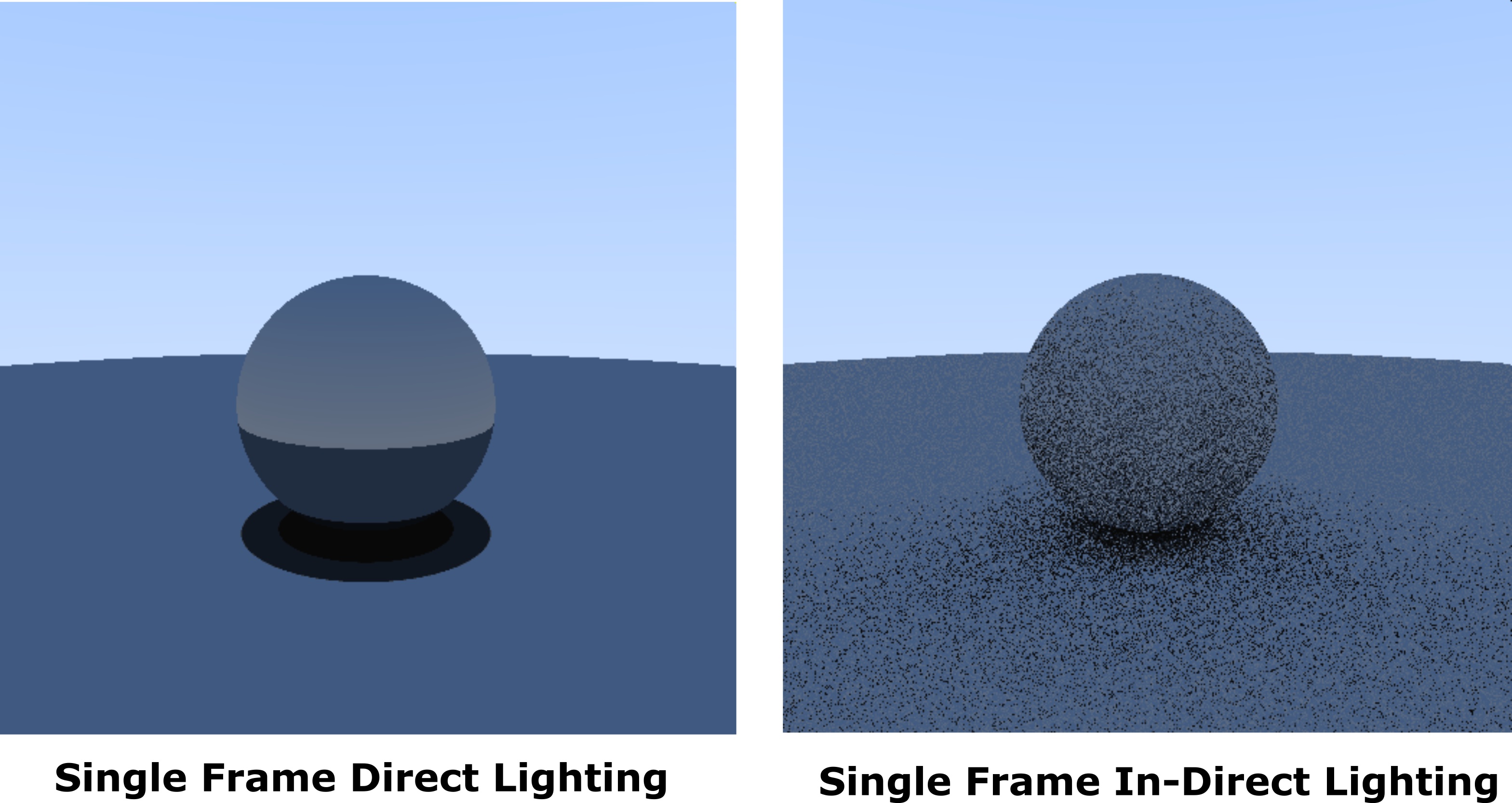
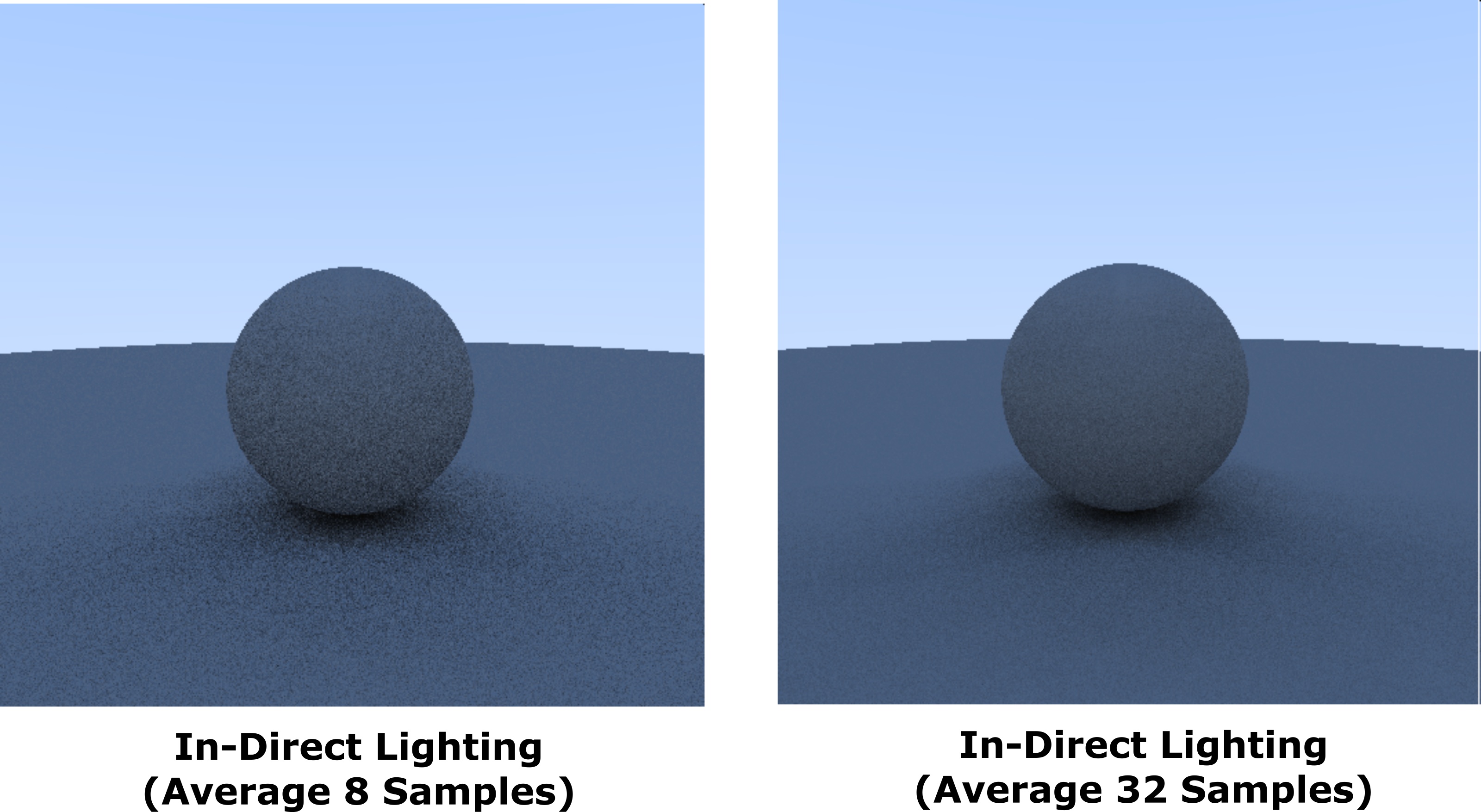
Indirect lighting refers to the light that bounces off surfaces in a scene and illuminates other areas, as opposed to direct light that comes straight from a light source. It plays a crucial role in simulating realistic lighting by capturing effects like global illumination, soft shadows, and color bleeding between surfaces. This type of lighting is often computationally expensive, as it involves tracing multiple rays and accounting for the multiple bounces of light within the scene.
Compare direct lighting with indirect lighting for the diffusion calculation.
Pseudo Code for Indirect Lighting Only:
Click here for details
// Function to trace a single bounce for indirect lighting
function TraceIndirectRay(rayOrigin, rayDirection, scene):
    // Trace the ray and return the intersection point if it hits an object
    intersection = TraceRay(rayOrigin, rayDirection, scene)

    if intersection is not null:
        // Calculate the surface properties (e.g., normal)
        surfaceNormal = intersection.normal

        // Randomly generate a new direction using the surface normal (**indirect vector**)
        newDirection = SampleDiffuseDirection(surfaceNormal) // e.g., RandomInHemisphere(..)

        // Recursively trace the indirect ray for global illumination
        indirectRadiance = TraceIndirectRay(intersection.position, newDirection, scene)

        // Multiply the indirect light by the material's reflectance and surface properties
        return indirectRadiance * material.albedo // Albedo represents the surface's reflectivity

    else:
        // If no intersection occurs (ray goes to infinity), return zero radiance
        return vec3(0.0, 0.0, 0.0) // No light contribution

// Main rendering loop for indirect lighting only
function RenderScene(scene, camera):
    // Loop through each pixel on the screen
    for each pixel in camera.screen:
        // Generate a primary ray from the camera to the scene
        rayOrigin = camera.position
        rayDirection = GenerateRayDirection(pixel)

        // Trace the primary ray and calculate indirect lighting
        radiance = TraceIndirectRay(rayOrigin, rayDirection, scene)

        // Store the resulting color in the image buffer
        image[pixel] = radiance

// Example of how to sample a new direction for diffuse reflection (Lambertian sampling)
function SampleDiffuseDirection(surfaceNormal):
    // Randomly sample a hemisphere around the surface normal using importance sampling
    randomPoint = RandomInHemisphere(surfaceNormal)
    return normalize(randomPoint)

// Example of ray tracing (simplified, for intersection and shading)
function TraceRay(rayOrigin, rayDirection, scene):
    // Perform intersection test with scene objects
    // Return the intersection details like position, normal, and material
    return intersectionDetails // If the ray intersects an object

// Main execution
scene = LoadScene("example_scene")
camera = SetupCamera()

RenderScene(scene, camera)
Example of a single frame direct lighting versus the indirect lighting for the reflection vector (indirect vector is calculated using a random halfsphere).
Take a large number of indirect samples using different random reflection vectors - add them together (for an average) to create a smooth result.